Page 99 - Contributed Paper Session (CPS) - Volume 1

CPS1158 Varun A. et al.
where
1  ' ' 
+
−1
S = ( Y − ( ij) X )( Y − ( ij) X ) (  ( ij) − ( ij) ) (  ( ij) − ( ij) )+ v 2
I
ij
2   ij ij ij ij 0 ij 0 ij  
ij n  n 
m − ij u ij
2
 d i0 −1 m i k ( ) 2 v     2 + u   1
ij 
ij
'
Y
P (T , Y | ( ij) , ij 2 , r , d , m )=  i=1    1   2  Y + 2 v +
ij
ij
i
ij
ij
B
T −1
i=1
j=1
    (b − a  u ) X ' X + I − 2
1
) (
 m  ij ij ij ij ij ij
ij n + ij u
−
'
−1
−1
)
−1
−1
 0 ( ij) ' I  0 ( ij) − (X ij ' Y + I  0 ( ij) )(X ' ij X + I ij −1 ) (X ij ' Y + I  0 ( ij      2
) 
ij
ij
ij
ij
ij
ij
T −m T −1
( Y | ( ij) , ij 2 , r , d , m )=    P (T , Y | ( ij) , ij 2 , r , d , m )
P
ij
ij
B
i
i
T 1 =1 T m =T m −1 +1

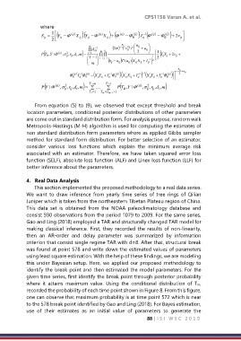
From equation (5) to (9), we observed that except threshold and break
location parameters, conditional posterior distributions of other parameters
are come out in standard distribution form. For analysis purpose, random walk
Metropolis-Hastings (M-H) algorithm is used for computing the estimates of
non standard distribution form parameters where as applied Gibbs sampler
method for standard form distribution. For better selection of an estimator,
consider various loss functions which explain the minimum average risk
associated with an estimator. Therefore, we have taken squared error loss
function (SELF), absolute loss function (ALF) and Linex loss function (LLF) for
better inference about the parameters.

4. Real Data Analysis
This section implemented the proposed methodology to a real data series.
We want to draw inference from yearly time series of tree rings of Qilian
Juniper which is taken from the northeastern Tibetan Plateau region of China.
This data set is obtained from the NOAA paleoclimatology database and
consist 930 observations from the period 1079 to 2009. For the same series,
Gao and Ling (2018) employed a TAR and structurally changed TAR model for
making classical inference. First, they recorded the results of non-linearity,
then an AR-order and delay parameter was summarized by information
criterion that consist single regime TAR with d=8. After that, structural break
was found at point 578 and write down the estimated values of parameters
using least square estimation. With the help of these findings, we are modeling
this under Bayesian setup. Here, we applied our proposed methodology to
identify the break point and then estimated the model parameters. For the
given time series, first identify the break point through posterior probability
where it attains maximum value. Using the conditional distribution of Tm,
recorded the probability of each time point shown in Figure 8. From this figure,
one can observe that maximum probability is at time point 572 which is near
to the 578 break point identified by Gao and Ling (2018). For Bayes estimation,
use of their estimates as an initial value of parameters to generate the
88 | I S I W S C 2 0 1 9