Page 108 - Contributed Paper Session (CPS) - Volume 2

CPS1443 Shogo H.N. et al.
e.g., Uchida and Yoshida (2012). The 2-dimensional latent process { } is
≥0
defined by the following SDE:

(1) (1) 1 2 1
d [ ] = ([ 1 3 ] [ ] + [ 5 ]) d + [ ] d , = [ ],

0
(2) 2 4 (2) 6 2 3 1

where { } is a 2-dimensional Wiener process. Our observation { ℎ =0,…,
}
≥0
is defined as
= + Λ 1/2 , = 0, … , ,
ℎ ℎ ℎ

where Λ is a 2 × 2 -dimensional positive semi-definite matrix, and
⋆
ℎ ∼ ... (, ). Let us set the parameters in the simulation by Λ = 10 −4 ,

2
2
6
⋆
⋆
= (1, 0.1, 1) , = (−1, −0.1, −0.1, −1, 1, 1) , = 10 , ℎ = 6.310 × 10 −5 ,

= 63.096, = 1.9, = 6172, = 162, Δ = 1.022 × 10 . The number of
−2

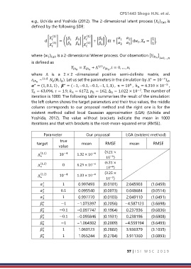
iteration is 1000. The following table summarises the result of the simulation:
the left column shows the target parameters and their true values, the middle
column corresponds to our proposal method and the right one is for the
existent method called local Gaussian approximation (LGA) (Uchida and
Yoshida, 2012). The value without brackets indicate the mean in 1000
iterations and that with brackets is the root-mean-squared error (RMSE).

Parameter Our proposal LGA (existent method)
true
target mean RMSE mean RMSE
value
−4
−4
Λ (1,1) 10 1.32 × 10 (3.21 ×
10 )
⋆
−5
(1,2) 0 6.29 × 10 (6.31 ×
−6
Λ ⋆ 10 )
−6
−4
−4
Λ (2,2) 10 1.33 × 10 (3.25 ×
10 )
⋆
−5
1 0.997493 (0.0101) 2.045903 (1.0459)
⋆
1
0.1 0.095540 (0.0073) 0.048684 (0.0514)
⋆
2
1 0.997770 (0.0103) 2.049110 (1.0491)
⋆
3
−1 −1.073397 (0.2056) −4.587123 (3.6698)
⋆
1
−0.1 −0.097747 (0.1964) 0.237936 (0.6836)
⋆
2
−0.1 −0.095846 (0.1931) 0.238196 (0.6808)
⋆
3
−1 −1.064302 (0.2009) −4.559194 (3.6493)
⋆
4
1 1.060123 (0.2802) 3.936379 (3.1035)
⋆
5
1 1.055244 (0.2784) 3.911360 (3.0893)
⋆
6
97 | I S I W S C 2 0 1 9