Page 121 - Contributed Paper Session (CPS) - Volume 2

CPS1458 KHOO W.C et al.
and finite variance  . The mixture operator ‘  ’ mixes two independent
2

random variables with the mixing weight  and −  respectively. The
1
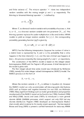
thinning (or binomial thinning) operator ‘ ’, is defined by

t X −1
  X t −1 =  i (2)
Y
i =1

Where Y is a Bernoulli random variable with probability of success  , that
i
is,  X − t 1 is a Binomial random variable with the parameter (X 1 − t  , ). This

thinning operator replaces the scalar multiplication in Box and Jenkins’ ARMA
models to yield an integer random variable. For z  1, the corresponding
probability generating function (pgf) is given by

−
) 
P (z = P 1 ( −  + ) z  + (1  )P (z )
t X t X − 1 t 

MPT(1) has the following interpretation. Suppose the number of crime in
a district town is represented by X and  is the probability that a crime
t
happens in the time interval t − 1,t ) , and the new criminal case happens at

time t , the process is mixed by the mixing weight of  and − respectively.
1
The construction of the MPT(1) model is based on the integer-valued
Autoregressive (INAR) and the Pegram’s AR processes. A brief description of
the model is given next.
The first integer-valued time series model was introduced by McKenzie
(1985), namely first order integer-valued Autoregressive (INAR(1)) model. The
INAR(1) process is in the form of


X =  X t−1 +  (3)
t
t

Where the random variable  X 1 − t is defined in Equation (2). However
the INAR(1) model can only accommodate self-decomposable distributions
(DSD) such as Poisson and negative binomial. For non DSD, see McKenzie
(1985). Many significant findings such as model generalization and properties
development of the INAR(1) model can be found in Joe (1996), Freeland (1998)
and Wei β (2008). Jacobs and Lewis (1987a, b) introduced a more general
discrete ARMA (DARMA) processes, which support not only DSD but any
discrete distribution. Pegram (1980) developed an Autoregressive Markov
chain model, which is similar to the Jacobs-Lewis’s approach. This has inspired
Biswas and Song (2009) to present a unified framework for stationary ARMA

110 | I S I W S C 2 0 1 9