Page 122 - Contributed Paper Session (CPS) - Volume 2

CPS1458 KHOO W.C et al.
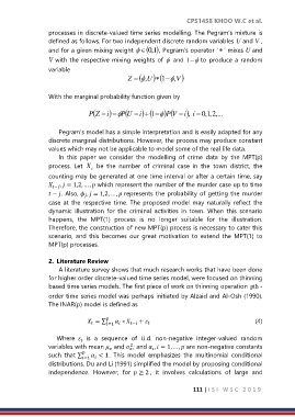
processes in discrete-valued time series modelling. The Pegram’s mixture is
defined as follows. For two independent discrete random variables U and V ,
and for a given mixing weight  ( ) 1,0 , Pegram’s operator ‘ ’ mixes U and
V with the respective mixing weights of  and −  to produce a random
1
variable

Z = ( U ,  ) (1  V , )
−

With the marginal probability function given by



+
i
P ( = i )= P ( = i ) (1− P V ), = , 2 , 1 , 0 ...
) ( = i
U
Z

Pegram’s model has a simple interpretation and is easily adapted for any
discrete marginal distributions. However, the process may produce constant
values which may not be applicable to model some of the real life data.
In this paper we consider the modelling of crime data by the MPT(p)
process. Let X be the number of criminal case in the town district, the
t
counting may be generated at one time interval or after a certain time, say
− , = 1,2, … , which represent the number of the murder case up to time
− . Also, , = 1,2, … , represents the probability of getting the murder

case at the respective time. The proposed model may naturally reflect the
dynamic illustration for the criminal activities in town. When this scenario
happens, the MPT(1) process is no longer suitable for the illustration.
Therefore, the construction of new MPT(p) process is necessary to cater this
scenario, and this becomes our great motivation to extend the MPT(1) to
MPT(p) processes.

2. Literature Review
A literature survey shows that much research works that have been done
for higher order discrete-valued time series model, were focused on thinning
based time series models. The first piece of work on thinning operation pth -
order time series model was perhaps initiated by Alzaid and Al-Osh (1990).
The INAR(p) model is defined as

= ∑ ∘ − + (4)

=1

Where is a sequence of i.i.d. non-negative integer-valued random

variables with mean and ; and , = 1, … , are non-negative constants
2

such that ∑ < 1. This model emphasizes the multinomial conditional

=1
distributions. Du and Li (1991) simplified the model by proposing conditional
independence. However, for ≥ 2 , it involves calculations of large and
111 | I S I W S C 2 0 1 9