Page 126 - Contributed Paper Session (CPS) - Volume 2

CPS1458 KHOO W.C et al.
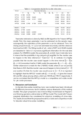
Table 4.1: Comparative studies for murder crime data
Model Parameter Estimates
α^ ϕ ^ ϕ ^ ϕ ^ ϕ ^ ϕ ^ ϕ ^ λ ^ AIC BIC
1
2
5
6
3
4
MPT(1) 0.1406 0.5630 0.3266 199.64 208.28
MPT(2) 0.1311 0.4305 0.4463 0.3484 196.66 208.19
MPT(3) 0.2705 0.2688 0.2431 0.4831 0.3337 192.64 207.05
MPT(3)* 0.3061 - - 0.6845 0.3133 189.48 198.12
MPT(4) 0.3340 0.2542 0.1504 0.2720 0.2565 0.3268 193.54 210.84

CINAR(1) 0.1259 0.2936 194.48 200.24
CINAR(2) 0.1709 0.6341 0.2793 194.79 203.44
CINAR(3) 0.2506 0.0001 0.00001 0.2557 191.75 203.29
CINAR(4) 0.2645 0.0000 0.0001 0.9501 0.2528 192.93 207.34

Parameter estimation is done by MLE via EM algorithm for Poisson MPT(p)
model. First, the mean parameter can be estimated via the sample mean,
subsequently, the estimation of the parameter can be obtained. Then, the
mixing proportions , = 1,2,3,4 are estimated recursively until the tolerance
^

level reaches 0.001. The fitting results of pth -order of MPT and CINAR models
are tabulated in Table 4.1. It provides significant information for the real data
analysis. For CINAR(3) model, the parameters and have trivial roles here.
^
^
2
1
It means that the possibility is low (almost not possible) for the murder case
to happen in the time interval  , − t t  1 and  , − t t  2 . In contrast, it is highly
possible that the murder case would happen in the time interval  , −  3 as
t t
= 0.99 (remember that for CINAR model, the parameter = 1 − − ).
^
^
^
^
1
2
3
3
Similar observation is made for the CINAR(4) model, where it can be noticed
that there is 95% that the murder case would happen in time interval  , −  3
t t
and another 5% that the murder case would occur in  , −tt  4 . It is important
to highlight that the MPT(3)* model with = 0 and = 0 gives the lowest
^
^
1
2
AIC and BIC values among others, which are 189.48 and 198.12 respectively. It
can be concluded that the MPT(p) model is a competitive and viable model
for pth -order processes.
5. Discussion and Conclusion
In discrete-time series modelling many new models have been introduced
to fit different phenomena. And to address various drawbacks of the existing
models. This paper proposed a new mixture AR(p) model based on Pegram’s
and thinning operators, abbreviated as MPT(p) model. The model with Poisson
marginal distribution has considered for empirical modelling of crime data.
The results showed that the proposed model is a viable and competitive model
for discrete-valued time series modelling.

115 | I S I W S C 2 0 1 9