Page 230 - Contributed Paper Session (CPS) - Volume 2

CPS1844 Reza M.
To illustrate the utility of such simultaneous display of the ECDFs, we
present the following examples where d = 100, s = 100 and nx = ny = 50.

2
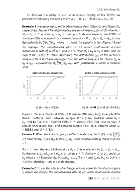
Example 1 We generate nx and ny observations from N(0,σx Id) and N(µ,σy Id),
2
respectively. Figure 1 Panel (a) displays the simultaneous plot of (2) when ∶
0
= , is true, with = = 1 = 0. As one expects, the ECDFs of
2
2

1
2
the three IPDs concentrate in a narrow band since ′ ∶ = = is true.

0
(L) (L) ()
Equivalently, = = where stands for equality in law. Figure 1 Panel

=
(b) displays the simultaneous plot of (2) under multivariate normal
distributions with = = 1 and µ = 1. Here, ∶ = is false, and we
2
2
2
1

0
expect the ECDFs to differ. Moreover, the distribution of the between
sample IPDs is stochastically larger than the within sample IPDs. Hence, =

(L)
= . Equivalently, = ≤ with probability 1 under a location

shift.

a) G1 = G2 ∼N(0,Id). b) G1 ∼N(0,Id) and G2 ∼N(1,Id).
Figure 1: Panel a: Empirical CDFs of sample IPDs (red, top), sample IPDs
(black, bottom), and between sample IPDs (blue, middle) when =
1
∼ℕ(0,Id). Panel b: Empirical CDFs of X sample IPDs (red, next to top), Y
2
sample IPDs (black, top), and between sample IPDs (blue, bottom) when G1
∼ ℕ(0,Id) and G2 ∼ ℕ(1,Id).
1
Lemma 2 When the X and Y groups differ in scale only; i.e. () = ( ),
2
1

we have min( , ) ≤ ≤ max( , ) with equality holding if and only if σ

= 1.
If σ = 1, then the result follows since = is equivalent to = = .

1
2
Furthermore, ≤ and ≤ when σ < 1. Similarly, ≤ and ≤

when σ > 1 Equivalently, ≤St ≤St if σ > 1 and ≤St ≤St if σ <

1 with probability 1 under a scale change.
Example 2 To see the effects of a change in scale, consider Panel (a) in Figure
2 where we display the simultaneous plot of (2) under multivariate normal
219 | I S I W S C 2 0 1 9