Page 40 - Contributed Paper Session (CPS) - Volume 2

CPS1414 Bashiru. I.I S. at el.
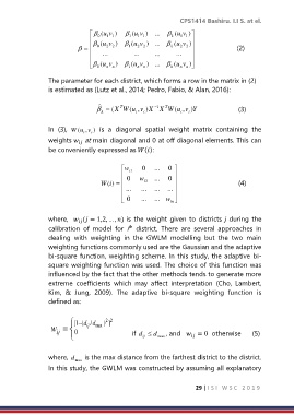
  0 ( vu 1 1 )  1 ( vu 1 1 ) ...  k ( vu 1 1  )
  ( vu )  ( vu ) ...  ( vu ) 
 =  0 2 2 1 2 2 k 2 2  (2)
 ... ... ... ... 
 
  0 ( vu n n )  1 ( vu n n ) ...  k ( vu n n ) 

The parameter for each district, which forms a row in the matrix in (2)
is estimated as (Lutz et al., 2014; Pedro, Fabio, & Alan, 2016):


 k = X ( T W u ( i v , i X ) 1 − X T W u ( i v , i Y ) (3)

In (3), W (u i ,v i ) is a diagonal spatial weight matrix containing the
weights at main diagonal and 0 at off diagonal elements. This can

be conveniently expressed as ():

w i1 0 ... 0 
 0 w ... 0 
W( i) =  i2  (4)
 ... ... ... ... 
 
 0 ... ... w in 

where, ( = 1,2, … , ) is the weight given to districts during the

th
calibration of model for i district. There are several approaches in
dealing with weighting in the GWLM modelling but the two main
weighting functions commonly used are the Gaussian and the adaptive
bi-square function, weighting scheme. In this study, the adaptive bi-
square weighting function was used. The choice of this function was
influenced by the fact that the other methods tends to generate more
extreme coefficients which may affect interpretation (Cho, Lambert,
Kim, & Jung, 2009). The adaptive bi-square weighting function is
defined as:

w ij =  1 [ −(d ij /d max 2 ] ) 2 if d  d max , and = 0 otherwise (5)
 0


ij

where, d is the max distance from the farthest district to the district.
max
In this study, the GWLM was constructed by assuming all explanatory

29 | I S I W S C 2 0 1 9