Page 35 - Contributed Paper Session (CPS) - Volume 2

CPS1409 Rahma F.
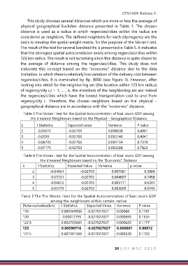
This study chooses several distances which are more or less the average of
physical geographical Euclidian distance presented in Table 1. The chosen
distance is used as a radius in which regencies/cities within the radius are
considered as neighbors. The defined neighbors for each city/regency are the
basis to develop the spatial weight matrix, for the purpose of the Moran I test.
The result of the test for several bandwidths is presented in Table 5. It indicates
that the strongest spatial autocorrelation exists among regencies/cities within
125 km radius. The result is not surprising since this distance is quite closed to
the average of distance among the regencies/cities. This study does not
elaborate this concept based on the “economic” distance due to the data
limitation, in which there is relatively low variation of the delivery cost between
regencies/cities. It is dominated by Rp. 8000 (see Figure 3). However, after
looking into detail for the neighboring set (the location within 125 km radius)
of regency/city , = 1, … , n, the members of the neighboring set are indeed
the regencies/cities which have the lowest transportation cost to and from
regency/city . Therefore, the chosen neighbors based on the physical –
geographical distance are in accordance with the “economic” distance.

Table 3 The Moran I test for the Spatial Autocorrelation of East Java’s GDP among
the k nearest Neighbours based on the Physical – Geographical Distance
k I Statistics Expected value Variance P value
2 -0.02611 -0.02703 0.008638 0.4961
3 -0.0259 -0.02703 0.005746 0.4941
4 -0.06795 -0.02703 0.004134 0.7378
5 -0.07175 -0.02703 0.003288 0.7823

Table 4 The Moran I test for the Spatial Autocorrelation of East Java’s GDP among
the k nearest Neighbours based on the “Economic” Distance
k I Statistics Expected Value Variance p value
2 -0.04661 -0.02703 0.007681 0.5884
3 -0.07331 -0.02703 0.004897 0.7458
4 -0.04873 -0.02703 0.003771 0.6381
5 -0.05179 -0.02703 0.003005 0.6743

Table 5 The The Moran I test for the Spatial Autocorrelation of East Java’s GDP
among the neighbours within certain radius
Distance/radius(km) I Statistics Expected Value Variance P value
110 0.000349908 -0.027027027 0.00088 0.1781
120 -0.00012795 -0.027027027 0.000693 0.1535
122.5 0.002733605 -0.027027027 0.000629 0.1177
125 0.00596716 -0.027027027 0.000601 0.08912
127.5 0.001391369 -0.027027027 0.000538 0.1103

24 | I S I W S C 2 0 1 9