Page 440 - Contributed Paper Session (CPS) - Volume 2

CPS1917 Trijya S.
∞
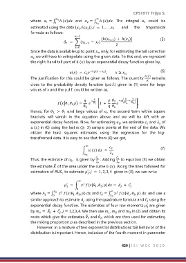
where = ∫ 0 ℎ () and = ∫ ℎ (). The integral could be
1
2
1

estimated using the data { , ℎ( )}, = 1, . . . , , and the trapezoidal

formula as follows:
−1
{ℎ( ) + ℎ( )} (5)
̂ = ∑( − ) +1
+1

1
2
=0
Since the data is available up to point only, for estimating the tail correction

we will have to extrapolate using the given data. To this end, we represent
2
the right-hand tail part of ℎ () by an exponential decay function given by,

() = − ( − ) , ≥ (6)

The justification for this could be given as follows. The quantity ℎ() remains

close to the probability density function (p.d.f.) given in (1) even for large
values of x and the p.d.f. could be written as,

− 2 −( 1 − 1 )
(| ) = 2 [1 + 1, 2, ].
1, 2,
2 1
Hence, for > nd large values of , the second term within square
1
2,

brackets will vanish in the equation above and we will be left with an
exponential decay function. Now, for estimating , we estimate and of
2

() in (6) using the last (≥ 3) sample points at the end of the data. We
obtain the least squares estimates using the regression for the log-
transformed data. It is easy to see that from (6) we get,

∞ (7)
∫ () =

Thus, the estimate of , is given by . Adding to equation (5) we obtain

2
̂
̂

the estimate of the area under the curve ℎ (). Along the lines followed for
̂
estimation of AUC, to estimate , = 1, 2, 3, 4 given in (3), we can write
′

∞
= ∫ (| , , ) = +
′

2
1

0
∞
where = ∫ 0 (| , , ) and = ∫ (| , , ) and use a

2

1
1
2

similar approach to estimate using the quadrature formula and using the

exponential decay function. The estimates of four raw moments are given
′

by = + , = 1,2,3,4. We then use , and in (2) and obtain its
̂
̂
1
2
3

roots which give the estimates and , which are then used for estimating
̂
̂
2
1
the mixing proportion p as described in the previous section.
However, in a mixture of two exponential distributions tail behavior of the
distribution is important. Hence, inclusion of the fourth moment in parameter
429 | I S I W S C 2 0 1 9