Page 96 - Contributed Paper Session (CPS) - Volume 2

CPS1442 Uzuke C.A. et al.
A test statistic for the null hypothesis of equation (i) based on W may be
developed by complete enumeration following the specifications in Equations
2 – 6. This approach is however tedious. A rather less cumbersome approach
based on the chi-square test for independence is adopted here.
−
+
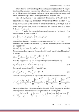
Now let t , t , and t be respectively the number of 1’s, 0’s and -1’s
0
j
j
j
obtained in the frequency distribution of the r values of these numbers in U ij
of Equation 2; that is, the number of times observations x in the jth level of
ij
factor B are greater than , equal to or less than the common median M for i =
1, 2, …, r; j = 1, 2, …, c
0
−
+
Let t , t and t be respectively the total number of 1’s, 0’s and -1’s in
all the c levels of factor B. that is
c c c
−
t ; t
t
t + =  j + − =  j − 0 =  j 0 = rc − t + − t (7)
t , t
j =i = j 1 = j 1
−
+
0
The total number of 1’s, -1’s and 0’sin the data set is t + t + t = rc
Note that the observed number of 1’s, -1’s and 0’s in the jth level of factor B
are respectively
−
+
−
O j 1 = t ;O 2 j = t and O 3 j = t 0 j = r − t + j − t (8)
j
j
j
The corresponding expected frequencies if the null hypothesis of Equation 1
is true are
rt + rt − rt 0 r (rc − t + t − − )
E = ; E = ; E = = (9)
j 1
rc 2 j rc j 3 rc rc
Also the proportions 1’s, -1’s and 0’s in the jth level of factor B are
t + t − t 0
−
P = ; P = ; P 0 = =1 − P + − P (10)
−
+
j j j j j
r r r
The overall proportion of 1’s, -1’s and 0’s are
t + t − t 0
−
−
P = ; P = ; P 0 = =1 − P + − P (11)
+
rc rc rc
Under the null hypothesis of equal factor B level effects the test statistic
 + − rt +  2  − − rt −  2  t 0 − rt 0  2



)
t
t
2
c
r
c
c
c






 2 =  (O ij − E ij =   j rc  +   j rc  +   j rc 
= i 1 = j 1 E ij = j 1 rt + = j 1 rt − = j 1 rt 0
rc rc rc
has approximately a chi-square distribution with 2(c-1) degrees of freedom.
This expression when simplified using Equation 10 and 11 yields 2
2
2
c
c
c
 2 = r  (P j + − P + ) + r  (P j − − P − ) + r  ( ( − P1 j + − P j − ) ( −− 1 P + − P − ))
+
−
−
+
= j 1 P = j 1 P = j 1 1 − P − P
85 | I S I W S C 2 0 1 9