Page 97 - Contributed Paper Session (CPS) - Volume 2

CPS1442 Uzuke C.A. et al.
r ( ( P − ( 1− P + − P − )) (P + − P + ) 2
c

= P + P − ( 1− P + − P − ) c 1 = j c j

2
2
+
+ P + ( 1− P + − P − ) (P j − − P − ) + P + P −  ( ( P j + − P + ) (P j − − P − )) )
1 = j 1 = j
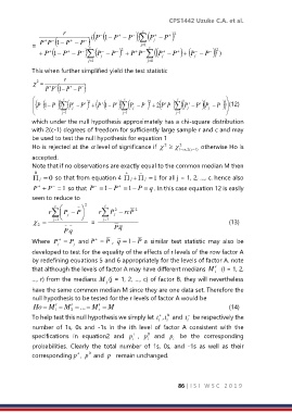
This when further simplified yield the test statistic
r
 2 =
−
( − P
P + P 1 + − P − )
 − − c + + 2 + + c − − 2 + − c + + − − 



( − P
2
+ P

 ( (  P 1 − P )) (P j − P ) ( + P 1 )) (P j − P ) ( P ) ( ( P j − P )(P j − P ))(12)
 = j 1 = j 1 = j 1 
which under the null hypothesis approximately has a chi-square distribution
with 2(c-1) degrees of freedom for sufficiently large sample r and c and may
be used to test the null hypothesis for equation 1
2
Ho is rejected at the  level of significance if  2   1− ( 2 ; c − ) 1 otherwise Ho is
accepted.
Note that if no observations are exactly equal to the common median M then
0 + −
 j = 0 so that from equation 4  j +  j = 1 for all j = 1, 2, …, c. hence also
+
−
P + + P − = 1 so that P =1 − P =1 − P = q . In this case equation 12 is easily
seen to reduce to
c  −  2 c
2
r  P j − P  r  P − rc P 2
j
= 
 2 = j 1 − −  = j 1 = (13)
P q P q
+
+
Where P = P and P = P , q =1 − P a similar test statistic may also be
j
j
developed to test for the equality of the effects of r levels of the row factor A
by redefining equations 5 and 6 appropriately for the levels of factor A. note
that although the levels of factor A may have different medians M  (I = 1, 2,
i
…, r) from the medians M (j = 1, 2, …, c) of factor B, they will nevertheless
j
have the same common median M since they are one data set. Therefore the
null hypothesis to be tested for the r levels of factor A would be
Ho = M = M =... = M = M (14)



1 2 r
+
−
To help test this null hypothesis we simply let t ,t and t be respectively the
0
i
i
i
number of 1s, 0s and -1s in the ith level of factor A consistent with the
+
−
specifications in equation2 and p , p and p be the corresponding
0
i
i
i
probabilities. Clearly the total number of 1s, 0s, and -1s as well as their
+
−
0
corresponding p , p and p remain unchanged.
86 | I S I W S C 2 0 1 9