Page 104 - Contributed Paper Session (CPS) - Volume 4

CPS2134 Yutaka Kuroki et al.
➢ Some predicted time-series plots together with predicting
performance measures are shown

For the first purpose, recall that we propose the following model:
7

, = ∑ , , + + ∑ + .
,

,
, ,
=1 =1
In order to obtain unbiased estimates of the OLS regression, it must be
assumed that error terms and regressors including factors must be
uncorrelated in both times-series and cross-sectional direction. This
assumption is known to the strictly exogenous assumptions, which seems too
strong to be hold. We need to perform some validity tests of our proposed
models are adequate or not. The following Fama-MacBeth regression,
together with GMM estimations are the powerful tools for panel time-series
analysis. Cochrane (2005) recommends keeping the number of test portfolios
to less than 10% of the number of observations in the GMM. Since we have
296 daily observations, we constructed 14 test portfolios based on their genre.

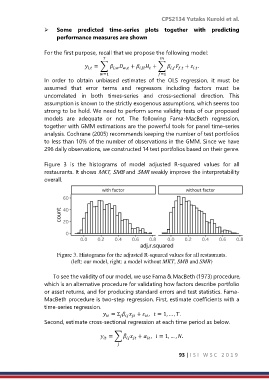
Figure 3 is the histograms of model adjusted R-squared values for all
restaurants. It shows MKT, SMB and SMR weakly improve the interpretability
overall.

Figure 3. Histograms for the adjusted R-squared values for all restaurants.
(left: our model, right: a model without MKT, SMB and SMR)

To see the validity of our model, we use Fama & MacBeth (1973) procedure,
which is an alternative procedure for validating how factors describe portfolio
or asset returns, and for producing standard errors and test statistics. Fama-
MacBeth procedure is two-step regression. First, estimate coefficients with a
time-series regression.
= Σ + , = 1, … , .

Second, estimate cross-sectional regression at each time period as below.
= ∑ + , = 1, … , .
̂

93 | I S I W S C 2 0 1 9