Page 109 - Contributed Paper Session (CPS) - Volume 4

CPS2135 Sumonkanti Das et al.
The estimated direct standard errors are reasonable for large domains, but
not always for small domains with only a few observed journey parts (even
ˆ
zero in some cases). In order to obtain more reliable se(Y it), a GVF model has
ˆ
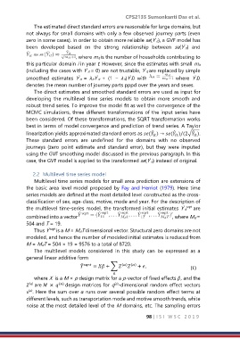
been developed based on the strong relationship between se(Y it) and
, where mit is the number of households contributing to

this particular domain i in year t. However, since the estimates with small mit
ˆ
ˆ
(including the cases with Y it = 0) are not trustable, Y it are replaced by simple
ˆ
ˆ
˜
ˆ
smoothed estimates Y it = λitY it + (1 − λit)Y i0. with where Y i0.
denotes the mean number of journey parts pppd over the years and sexes.
The direct estimates and smoothed standard errors are used as input for
developing the multilevel time series models to obtain more smooth and
robust trend series. To improve the model fit as well the convergence of the
MCMC simulations, three different transformations of the input series have
been considered. Of these transformations, the SQRT transformation works
best in terms of model convergence and prediction of trend series. A Taylor
linearization yields approximated standard errors as ( ) → ( )/(2√ ).
̂
̂
̂

These standard errors are undefined for the domains with no observed
journeys (zero point estimate and standard error), but they were imputed
using the GVF smoothing model discussed in the previous paragraph. In this
case, the GVF model is applied to the transformed se(Y it) instead of original.
ˆ

2.2 Multilevel time series model
Multilevel time series models for small area prediction are extensions of
the basic area level model proposed by Fay and Herriot (1979). Here time
series models are defined at the most detailed level constructed as the cross-
classification of sex, age-class, motive, mode and year. For the description of
ˆ sqrt are
the multilevel time-series model, the transformed initial estimates Y it
combined into a vector , where Md =
504 and T = 19.
Thus Y ˆsqrt is a M = MdT dimensional vector. Structural zero domains are not
modeled, and hence the number of modeled initial estimates is reduced from
M = MdT = 504 × 19 = 9576 to a total of 8720.
The multilevel models considered in this study can be expressed as a
general linear additive form

̂

= + ∑ () () + , (1)

where X is a M × p design matrix for a p-vector of fixed effects , and the
(α)
(α) are × () design matrices for q -dimensional random effect vectors
v . Here the sum over α runs over several possible random effect terms at
(α)
different levels, such as transportation mode and motive smooth trends, white
noise at the most detailed level of the M domains, etc. The sampling errors

98 | I S I W S C 2 0 1 9