Page 207 - Contributed Paper Session (CPS) - Volume 4

CPS2182 Lynne Billard et al.
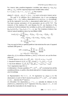
For interval data, predictor/regression variables take values = [ , ],

with < , and the response/dependent variable takes values

= [ , ], < , = 1, … , , = 1, … , . The model is

= +
′
where = ( , , … , ), = (1, , … , ) and ϵ is the error interval vector.
′
′
1
1

0
The goal is to partition the observations into non-overlapping
clusters, = ( , … , ) , with observations in and = . Accordingly,

1

we fit the regression line to the n, observations within each , = 1, … , .

The least squares estimators of the parameters are = (′) ′ . The
−1
elements of the matrices ′ , and likewise for ′ , are functions of the
covariance functions between two variables and with realizations =

[ , ] and = [ , ], = 1, … , , say. This covariance between two

interval-valued variables is given by (see Billard, 2008)

1
̅
̅
̅
̅
( , ) = ∑[2( − )( − ) + ( − )( − )

6
=1
̅
̅
̅
̅
+ ( − )( − ) + 2( − )( − )] ,

1
̅
= ∑( + )

2
=1
Thus, we want to find an optimal partition that minimizes the sum of squared
residuals (SSR) given ,

2
2
= ; ̂ ∑ ∑ = ∑ ∑ ,

=1 ∈ =1 =1
= ( , ̂ ) = ( , )
′

1
where ( , ̂ ) is a distance between and ̂ . In this work, we use the three

distances

1. Center distance: ( , ) = ∑ | − | , 1 = ( + )/2;
2
1

2
1
=1
2. Hausdorff distance: ( , ): ∑ max {| 1 − 2 |, | 1 − 2 |}
2

1
=1
3. City-block distance: ( , ) = ∑ [| 1 − 2 |, | 1 − 2 |].
2
1

=1
The -regressions algorithm is:
(0)
(i) Initialization: Choose a partition (0) = ( 1 (0) , … , ) randomly from all the
possible partitions, or partition the whole data set to clusters based on some
prior knowledge.

(ii) Representation: For = 1, … , , fit regressions = + to the
′

(1)
observations in each of the K clusters for partition (1) = ( 1 (1) , … , ) where
= 0,1, …, denotes the iteration.
ℎ
(iii) Allocation: For observation , = 1, … , , calculate its distance to its

prediction obtained by its regression line ( , ), = 1, … , , and
′ ̂
ℎ

1

allocate the observation to its closest line; i.e,
196 | I S I W S C 2 0 1 9