Page 214 - Contributed Paper Session (CPS) - Volume 4

CPS2192 Laurent D. et al.
1
̃ ̃
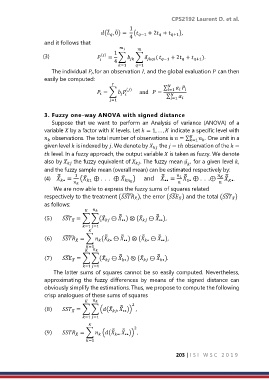
( , 0) = ( −1 + 2 + +1 ),

4
and it follows that

(3) () = 1 ∑ ∑ ( + 2 + ).
4 −1 +1
=1 =1
The individual ,for an observation , and the global evaluation can then

easily be computed:
∑
= ∑ () and = =1

∑
=1 =1
3. Fuzzy one-way ANOVA with signed distance
Suppose that we want to perform an Analysis of variance (ANOVA) of a
variable by a factor with levels. Let = 1, … , indicate a specific level with
observations. The total number of observations is = ∑ . One unit in a

=1
given level is indexed by . We denote by the − ℎ observation of the −

ℎ level. In a fuzzy approach, the output variable is taken as fuzzy. We denote
also by the fuzzy equivalent of . The fuzzy mean µ , for a given level ,

and the fuzzy sample mean (overall mean) can be estimated respectively by:
̅ 1 ̅ 1 ̅ ̅
̃
̃
̃
̃
̃
̃
(4) • = ( 1 ⊕ . . . ⊕ ) and = ⊕ . . .⊕ •·
1•
••

We are now able to express the fuzzy sums of squares related
̃
̃
̃
respectively to the treatment ( ̅), the error ( ̅) and the total ( ̅)

as follows:

̅
̅
̃
̃
̃
̃
̃
(5) ̃ = ∑ ∑( ⊖ ) ⊗ ( ⊖ ),
••

••
=1 =1

̅
̅
̅
̅
̃
̃
̃
̃
̃
(6) ̃ = ∑ ( ⊖ ) ⊗ ( ⊖ ),
••
•
•

••

=1

̅
̅
̃
̃
̃
̃
̃
(7) ̃ = ∑ ∑( ⊖ ) ⊗ ( ⊖ ).
•
•

=1 =1
The latter sums of squares cannot be so easily computed. Nevertheless,
approximating the fuzzy differences by means of the signed distance can
obviously simplify the estimations. Thus, we propose to compute the following
crisp analogues of these sums of squares

2
̅
(8) ̃ = ∑ ∑ (( , )) ,
̃
̃

••

=1 =1
2
̅
̅
(9) ̃ = ∑ (( , )) ,
̃
̃
•

••

=1
203 | I S I W S C 2 0 1 9