Page 279 - Contributed Paper Session (CPS) - Volume 4

CPS2224 Habshah Midi et al.
2
with cut off point of RDF taken as c with
r

Tr (S 2 ) { (S )} 2
Tr
c = m and r = m
Tr (S m ) Tr (S m 2 )
where Sm is the scatter matrix.

ˆ
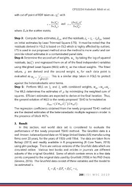
Step 3: Compute beta estimates,  and the residuals, ˆ  y − x  = ' ˆ based
LTS it it it LTS
on initial estimates by Least Trimmed Square (LTS). It must be noted that the
residuals derived in FGLS is based on OLS which is highly affected by outliers.
LTS is used in our proposed method since the method is more useful and can
provide robust estimates in a contaminated panel data.
Step 4: Determine the second set of weights, W by taking the log of squared
H
residuals, ln( ) and regressed them on all of the fixed independent variables
ˆ 
2
it
using Weighted Least Square (WLS) with W as the robust weights. The fitted
O
values, ˆ g are derived and the second weight, W for each data point is
H
evaluated as W = 1 . This is a similar step taken in FGLS to protect
H exp(g ˆ)
against the heteroskedastic error terms.

Step 5: Perform WLS on y and x with combined weights, W HO = W  H W .
it
it
O
The WLS determines the estimates of  by minimizing the weighted sum of
squares. Efficient estimates are expected to derive at the final iteration. Thus,
the general solution of WLS to the newly proposed TSHO is formulated as
)
−
1
 TSHO = ( X W X ) ( X W Y .
'
'
HO
HO
The regression coefficients obtained from the newly proposed TSHO method
are the desired estimates of the heteroskedastic multiple regression model in
the presence of block HLPs.

3. Result
In this section, real world data set is considered to evaluate the
performance of the newly proposed TSHO method. The Grunfeld data is a
well-known, balanced panel data on 10 large United States (US) manufacturing
firms over 20 years, for the years of 1935 until 1954. The data are taken from
Baltagi (2013) and readily available in R programming (R Core Team, 2013)
using plm package. There are various versions of the Grunfeld data which are
circulated online. Various text books and articles in journals use different
subsets of the original Grunfeld. Some of which contain errors in a few data
points compared to the original data used by Grunfeld (1958) in his PhD thesis
(Greene, 2016). The Grunfeld data consist of three variables and the model to
be estimated is
I =  +  1 it  2 C + 
F +
it
it
0
it
268 | I S I W S C 2 0 1 9