Page 252 - Contributed Paper Session (CPS) - Volume 6

CPS1909 Retius C. et al.
In this paper, we utilize the mean excess plot and the parameter stability
plot for threshold selections.

Pearson type-IV distribution
The generalized family of frequency curves, now known as the Pearsonian
system of curves, was first developed by Karl Pearson (Cheng, 2011). The
Pearsonian family includes members such as the normal, student-, F, gamma,
beta, inverse Gaussian, Pareto and Pearson type-IV distributions. The
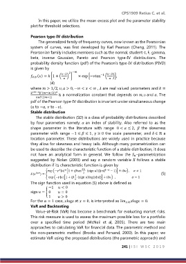
probability density function (pdf) of the Pearson’s type-IV distribution (PIVD)
is given by −
2
() = [1 + ( − ) ] × exp [−tan −1 ( − )],

(4)
where > 1 2, , > 0, −∞ < < ∞ , are real valued parameters and =
⁄
2 2−2 |Γ(− 2)| 2 is a normalization constant that depends on , and . The
⁄
(2−1)
pdf of the Pearson type-IV distribution is invariant under simultaneous change
( to −, to – ).
Stable distribution
The stable distribution (SD) is a class of probability distributions described
by four parameters namely: an index of stability. Also referred to as the
shape parameter in the literature with range 0 < ≤ 2, the skewness
parameter with range −1 ≤ ≤ 1, ≥ 0 the scale parameter, and ∈ ℝ a
location parameter. These distributions are widely used in practice because
they allow for skewness and heavy tails. Although many parametrization can
be used to describe the characteristic function of a stable distribution, it does
not have an analytical form in general. We follow the -parametrization
0
suggested by Nolan (2003) and say a random variable follows a stable
distribution if its characteristic function is given by
exp (− || [1 + tan (sign )(|| 1− − 1)] + ) , ≠ 1

( ) = { 2 (5)
2
exp (−|| [1 + (sign )log (||)] + ) , = 1

The sign function used in equation (5) above is defined as
−1 < 0
sign = { 0 = 0
1 > 0
For the = 1 case, log at = 0, is interpreted as lim ↓0 log = 0.
VaR and Backtesting
Value‐at‐Risk (VaR) has become a benchmark for evaluating market risks.
This risk measure is used to assess the maximum possible loss for a portfolio
over a specified time period (McNeil et al, 2005). There are two main
approaches to calculating VaR for financial data. The parametric method and
the non‐parametric method (Brooks and Persand, 2000). In this paper, we
estimate VaR using the proposed distributions (the parametric approach) and

241 | I S I W S C 2 0 1 9