Page 143 - Special Topic Session (STS) - Volume 2

STS474 Takaki S. et al.
′
and pre-determined before analysis. For parameters (, , , , ) , spatial

parameters, and , describes spatial interactions of return series and
, and are GARCH parameters and specify volatility behaviors. The

2
positivity of is ensured by the following sufficient restrictions > 0, ≥

,
0, ≥ 0, and the sum + < 1 for stationarity. Moreover, we assume|| +

|| < 1 to guarantee the existence of the model.
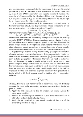
Let us consider the volatility matrix for SARMA-GARCH models. From (3),
the variance matrix of , Γ , is a diagonal matrix whose components are
2
,

that is Γ = ( , … , ). From equations (1) and (2),

,
1,
−1
−1
= ( − ) ( − ) .

Therefore, the volatility matrix for SARMA-GARCH models, ∑ , are

−1
−1
−1
∑ = ( − ) ( − ) Γ ( − ) ′−1 ( − )′ , (4)

2
where is an identity matrix. Volatility changes over time, so the volatility
,
matrix for SARMA-GARCH models expresses time-varying volatility structures
in financial instruments and can capture dynamic correlations. Moreover, the
spatial weight matrix in (4) expresses cross-sectional correlation between
observations and plays important role to reduce the number of parameters for
cross-sectional correlation and to overcome the curse of dimensionality.
A spatial weight matrix is usually determined by geographical information
of spatial data and predetermined such as first-order contiguity relation or
inverse distance between observations. However, { } are financial data and
,
don't include geographical information. Therefore, we need to determine
financial distances to make a spatial weight matrix. Some author have
proposed spatial weight matrix based on financial distance calculated from
financial statement data such as dividend yields or market capitalizations.
Here, we propose a method to make spatial weight matrices by multiple
regression models with backward stepwise model selection procedures. It
begins with the full least squares model containing all − 1 explanatory
variables.

= + ∑ + ,
0
,
,
,
≠
where follows an i.i.d standard normal distribution. Then, we iteratively
,
removes the least useful explanatory variables, one-at-a-time. Details are
given as follows:
1. Apply the OLS methods to the full model and obtain t-values for
explanatory variables.
2. Remove the explanatory variable whose t-value is the minimum values in
all t-values and not statistically significant.
3. Apply the OLS methods to the model contains all but one of the
explanatory variables in step 2.
132 | I S I W S C 2 0 1 9