Page 145 - Special Topic Session (STS) - Volume 2

STS474 Takaki S. et al.
2
where , = ,0 + 2 + 2 can be evaluated recursively.
,2 ,−1
,−1
Maximizing this with respect to , and , we have the estimators of GARCH

parameters.

4. Real data analysis
We examine empirical properties of SARMA-GARCH models by applying
daily return data of the U.S markets to demonstrate practical performances of
volatilities and co-volatilities identified by SARMA-GARCH models. Moreover,
we show prediction performance and dynamic spillover effect of shock.
We apply the SARMA-GARCH model to daily returns of the S&P 500 stock
price data, that is the returns {, } are computed as 100( − −1 ),

where is the closing price and t is the time index referring to trading day t.

The sampling period stars on April 1st, 2002 and ends on July 4th, 2016 for a
total of 3500 returns. Moreover, we sample data for prediction from July 5th,
2016 to December 30, 2016. The number of firms are 395. Spatial wight
matrices are made in accordance with the manner written in section 2. Here,
the critical value is 1.96.
We adopt constant conditional correlation (CCC) models as a benchmark.
Let = ( , … , ) be a n-dimensional vector process. CCC models are
,
1,

represented by the following equations
= 1

2
∑ ,

∑ = ( , … , ),
2
2

1,
,
= + 2 + 2 , = 1, … ,
,
,−1
,−1

where ∑ is a diagonal matrix with as th diagonal element, and
2

,
unobservable random vector with mean equal to 0 and variance-covariance
equal to = ( , , ). CCC models assume the correlation matrix is constant.

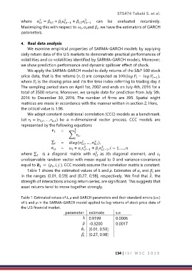
Table 1 shows the estimated values of λ and ρ. Estimates of and are

̂
in the ranges [0.01, 0.59] and [0.27, 0.98], respectively. We find that , the
strength of interactions among return series, are significant. This suggests that
asset returns tend to move together strongly.

Table 1: Estimated values of λ, ρ and GARCH parameters and their standard errors (s.e.)
of λ and ρ in the SARMA-GARCH model applied to log returns of stock price data of
the U.S financial market.
parameter estimate s.e
λ 0.9199 0.0006
̂ -0.3200 0.0017
̂ [0.01, 0.59]

̂
[0.27, 0.98]

134 | I S I W S C 2 0 1 9