Page 149 - Special Topic Session (STS) - Volume 2

STS474 Gigih F. et al.
values reported declined from -3.5% in 2008 to -33.1% in 2009 (MOF Press
Release, 2012).
Kawai and Takagi (2009) have shown that this occurred by the increasing
of Japan’s export to gross domestic product (GDP) ratio and trade openness.
Due to the declining of demand from US, then Japan had faced lower total
export. This decline is also affected financial institutions’ core profitability from
trade credit and financing as the regional capital is not kept up the increasing
off risk asset (BOJ Financial System Report, 2008). Demirer et al. (2017) also
show that the Japanese banks have strong connection globally impacted the
spread volatility across bank stocks, especially with US banks.
In this research, we conducted further investigation for the impact of
Lehman’s shock towards US and Japan regional economic growth. By using
this approach, we got a detailed illustration of how the shock transmitted
within country.

2. Methodology
2.1 Data and Target Variable
We used the real gross regional product (GRP) based on production
approach as the main dataset. The United States data were retrieved from
regional statistics in Bureau Economic Analysis (BEA) and we apply quarterly
nd
st
data from 1 Quarter of 2005 until 2 Quarter of 2018 for 51 states (including
District of Columbia). On the other hand, for Japan we use annually GRP data
from Economic and Social Research Institute, Cabinet Office for 47 prefectures
from 2001 until 2014.
Based on Reinhart & Rogoff (2008) and Bank for International Settlement
st
(BIS) Report (2009) we select the 1 quarter of 2008 as the breakpoint in the
US. On the other hand, following Filardo et al. (2009) and Kawai & Takagi
(2009), we select 2008 as the breakpoint for Japan regional data.

2.2 Empirical Model
2.2.1 Spatially-Independent Model
Our focus in this research is to observe the behavior of regional economic
growth fluctuation. This approach allowed us to identify before and after shock
conditions and observed which area had a recovery. Therefore, we analyze the
regional transitory, by observing the time-trend of regional economic growth
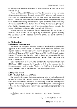
before and after crisis by using ordinary least-square (OLS) regression (Greene,
2012),

∗
∗
∗
2
∗
ln ( , ) ≡ , = + + ( + )( > ) + , , , ∼ (0, ) for ≤

,−1

∗ 2
∗
, ∼ (0, ) for > (1)

138 | I S I W S C 2 0 1 9