Page 150 - Special Topic Session (STS) - Volume 2

STS474 Gigih F. et al.
is GRP for states = 1, … , at time period = 1, … , and ln( ⁄ ,−1 ) is
,
,
regional economic growth, and represents exogenously selected breakpoint.
∗
Here, are intercept and is time trend component before crisis. Similarly,

∗
∗
( + ) and ( + ) are defined after crisis.

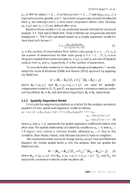
Based on those models in (1), we conducted several methods for structural
analysis: 1) F-Test; and 2) Wald-test. These methods use exogenously selected
∗
breakpoint, . The F-test calculated based on a simple regression model for
time trend with known ,
∗
= [ 1 − ( 2 + 3 )]/ (2)
( 2 + 3 )/( 1 + 2 −2)
∗
is the number of observations from before crisis group ( = 1, … , ), is
2
1
the number of observations for after crisis group ( = + 1, … , ). is sum
∗
1
of square residual from combined data ( + ), and are sum of squared
3
2
1
2
residual from and respectively. is the number of parameters.
1
2
To provide further evidence for structural change at breakpoint , we also
∗
adopt the Jouini & Boutahar (2004) and Greene (2012) approach by applying
the Wald test,
′
−1
̂
̂
2
̂
= ( − ) ( + ) ( − ) ~ (3)
̂
̂
̂

2

1
2

∗ ′
where = ( , ) and = ( + , + ) are used for spatially-
∗
′

̂
independent model in (1). and are asymptotic covariance matrices under
̂
2
1
null hypothesis: = and alternative hypothesis: ≠ respectively.

2.2.2 Spatially-Dependent Model
To include the neighboring relations as a factor for the analysis, we extend
equation (1) into spatial autoregressive model as follows,
∗
∗
∗
∗
, = + + ∑ ≠ , + ( + + ∑ ≠ , )( > ) + , ,

2
∗
, ∼ (0, ) for ≤

, ∼ (0, ) for > (4)
∗ 2
∗

∗
where and + represents the spatial regression coefficients before and

after crisis. The spatial relationship calculated by conditions = 0, and =

1 if region and shares a common border, otherwise = 0. Due to this

condition, then Alaska, Hawaii, and Okinawa became to have no neighbor.
We conducted similar structural change test by using F-Test and Wald test.
Equation (4) include spatial factor into the analysis, then we update the

Wald test into,
−1
′
̂
̂
̂
̂
2
̂
̂
= ( , − ) ( 1, + ) ( , − ) ~ (5)
,
,
3
2,
̂
̂
∗
∗ ′
′
∗
where , = ( , , ) and , = ( + , + , + ) . and are
2,

1,

asymptotic covariance matrices under equation (4).

139 | I S I W S C 2 0 1 9