Page 221 - Special Topic Session (STS) - Volume 2

STS486 R. Ayesha A. et al.
the true level of variation is at the group level (Guimarães and Lindrooth,
2007). Let be a × × design array containing covariate information,
with entries . We use to represent the K-length vector of covariates

associated with group g and choice j. The multinomial probabilities are

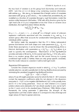
modelled as a function of covariates through a logit formulation. Under the
random utility framework (McFadden, 1974) with utility function given by the
right hand side of (1) plus independent errors that follow an extreme value
distribution, the logit formulation follows directly.

log ( ) = + ,

1−
(1)

for = 1, … , = 1, … , , where is a K-length vector of unknown
regression coefficients associated with the covariates in and is a
random group effect that accounts for unobservable heterogeneity among
individuals within a group.
We further make the assumption that the ’s follow independent
gamma distributions with both shape and scale parameters , > 0.

Under these assumptions, it can be shown that the probabilities follow a

Dirichlet distribution with parameters = ( −1 , … , −1 ), where is
1

used to quantify the overdispersion. Maximization of the log-likelihood
provides estimates of β and . In the special case that = 0 for all and ,

there is no random group effect and the DM model reduces to a group
conditional logit model. If, further, there are only group-specific covariates,
then the model reduces to a standard multinomial logit model.

Regularized DM regression
Consider the constant dispersion model in which = ∀ . To perform

variable selection, we add a penalty term to the log-likelihood and proceed by
minimizing the penalized (negative) log-likelihood function:
∗ ̃
̃
∗
ℓ ( , ) = − ℓ( ) + ℐ( ),
∗

where is an M-length parameter vector for which the first K = M–1 elements
∗
contain the regression coefficients while the last element is the dispersion
parameter , − ℓ( ) is the negative DM likelihood, ℐ( ) is the penalty term,
∗
∗
̃
and > 0 is the tuning parameter. Since our main interest is in a sparse
solution where some elements of are shrunk exactly to zero, we let ℐ( )
∗
∗
be the L1-norm, which is the standard lasso (Tibshirani, 1996). Within a lasso
̃
framework, the tuning parameter determines the strength of the
̃
regularization such that smaller values of correspond to less shrinkage and
̃
larger values of lead to sparser solutions.

210 | I S I W S C 2 0 1 9