Page 288 - Special Topic Session (STS) - Volume 3

STS544 Jonathan W. et al.

where = ( , … , ) , denotes an nx1 vector of observed variables,

1

denotes quarters, and denote nxn matrices of constant parameters (or
functions of constant “deeper” parameters), = ( , … , ) denotes an

1
nx1 vector of unobserved disturbances, and superscript T denotes vector or
matrix transposition. We assume (a) that is a sub-lower triangular matrix
with all elements on or above the principal diagonal equal to zero and (b) that
the disturbance covariance matrix is the identity matrix, ∑ = 1 . The

parameter elements of A, B, and ∑ are identified and estimated efficiently

(unbiasedly with minimum variance) by sequentially applying OLS to eqution
(1), equation by equation, from top to bottom.
The structure of coefficient matrix A reflects the Granger-causal ordering
of the variables in induced by the order in which they are observed in a

quarter. Thus, in is observed first in quarter t, is observed
2

1
second in quarter t, and so on. Forecasting with estimated equation (1) is
similarly
sequenced: is forecast using the first equation, is then forecast using
1
2
the second equation and the previously computed forecast of , and so on.
1
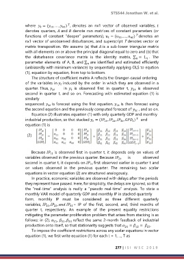
Equation (2) illustrates equation (1) with only quarterly GDP and monthly
industrial production, so that stacked = ( , , , ) and

2

1
3

equation (1) is

(2)

Because is observed first in quarter t, it depends only on values of
1
variables observed in the previous quarter. Because is observed
2
second in quarter t, it depends on first observed earlier in quarter t and
1
on values observed in the previous quarter. The remaining two scalar
equations in vector equation (2) are structured analogously.
In practice, economic variables are observed with delays after the periods
they represent have passed. Here, for simplicity, the delays are ignored, so that
the “real-time” analysis is really a “pseudo real-time” analysis. To state a
monthly VAR model of quarterly GDP and monthly IP in stacked quarterly
form, monthly IP must be considered as three different quarterly
variables, , , = IP of the first, second, and, third months of
3
2
1
quarter t, respectively. An example of the present equality restrictions
mitigating the parameter proliferation problem that arises from stacking is as
follows: in (2), , , reflect the same 2-month feedback of industrial
12
23
21
production onto itself, so that stationarity suggests that 21 = 12 = .
23
To impose the coefficient restrictions across any scalar equations in vector
equation (1), we first write equation (1) for each t = 1, ..., T as
277 | I S I W S C 2 0 1 9