Page 292 - Special Topic Session (STS) - Volume 3

STS544 Jonathan W. et al.
at least considering their natural provenance from stationarity, their rejection
should motivate thinking about why a considered model may or may not be
misspecified.

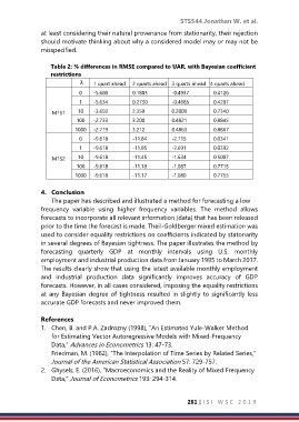
Table 2: % differences in RMSE compared to UAR, with Bayesian coefficient
restrictions
λ 1 quart ahead 2 quarts ahead 3 quarts ahead 4 quarts ahead
0 -5.680 0.1883 -0.4937 0.4126
1 -5.634 0.2730 -0.4685 0.4207

M1S1 10 -3.692 2.359 0.2009 0.7340
100 -2.733 3.200 0.4821 0.8845
1000 -2.719 3.212 0.4863 0.8867
0 -9.618 -11.84 -2.715 0.0341
1 -9.618 -11.85 -2.691 0.0392
M1S2 10 -9.618 -11.45 -1.634 0.5007
100 -9.618 -11.18 -1.087 0.7715
1000 -9.618 -11.17 -1.080 0.7755

4. Conclusion
The paper has described and illustrated a method for forecasting a low
frequency variable using higher frequency variables. The method allows
forecasts to incorporate all relevant information (data) that has been released
prior to the time the forecast is made. Theil-Goldberger mixed estimation was
used to consider equality restrictions on coefficients indicated by statonarity
in several degrees of Bayesian tightness. The paper illustrates the method by
forecasting quarterly GDP at monthly intervals using U.S. monthly
employment and industrial production data from January 1995 to March 2017.
The results clearly show that using the latest available monthly employment
and industrial production data significantly improves accuracy of GDP
forecasts. However, in all cases considered, imposing the equality restrictions
at any Bayesian degree of tightness resulted in slightly to significantly less
accurate GDP forecasts and never improved them.

References
1. Chen, B. and P.A. Zadrozny (1998), “An Estimated Yule-Walker Method
for Estimating Vector Autoregressive Models with Mixed-Frequency
Data,” Advances in Econometrics 13: 47-73.
Friedman, M. (1962), “The Interpolation of Time Series by Related Series,”
Journal of the American Statistical Association 57: 729-757.
2. Ghysels, E. (2016), "Macroeconomics and the Reality of Mixed Frequency
Data," Journal of Econometrics 193: 294-314.

281 | I S I W S C 2 0 1 9