Page 290 - Special Topic Session (STS) - Volume 3

STS544 Jonathan W. et al.
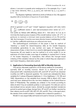
where is an error or pseudo error analogous to ̅. For example, if q = 1 and
̅ has three elements, then, ̅ , ̅ ̅ are restricted by ̅ = ̅ =
1
1
3
2
3
[1, 0, −1].
The Bayesian tightness restrictions work as follows in OLS. We append
equation (8) to the bottom of equation (7) and obtain

(9) [ ] = [ ] ̅ + [ ],
̅
̅
̅
0

which in general is a (nT+q)x1 “mixed” regression equation with data matrix
̅
̅

[ ], coefficient vector ̅, and real-and-pseudo-error vector (̅ , ) .
0
OLS works as follows with differing values of λ . OLS sets ̅ to ̅ ̈ so as to
minimize the least squares measure of the overall residual vector, (̅ ̈ , ̂ ) , in

̅
particular, to maintain a minimum least squares balance of ̅ ≅ ̅ and 0 ≅
λR̅. As λ increases, ̅ ̈ must be ever more directed toward maintaining 0 ≅ λR̅
so that the coefficient restrictions are enforced ever more.
The methodological contribution of the paper is that its method of
“stacking” a model for mixed-frequency data at the lowest frequency
immediately generalizes to any number and types of frequencies of
observation of data. In fact, there’s no need to distinguish among observation
frequencies. All one needs to use the method is to write model (1) (or an
extension of it that includes more lags of variables) in stacked form in terms
of the lowest frequency of observation, that reflects the Granger-causal
ordering of the variables induced by the order in which they are observed in
each lower-frequency observation period.

3. Application to Forecasting Quarterly GDP at Monthly Intervals
This section discusses application of the above method to forecasting
quarterly GDP at monthly intervals. Model (1) is defined in terms of
employment (EP), industrial production (IP), and GDP. EP and IP are observed
monthly and GDP is observed quarterly. The model was estimated for these
variables for 5 values of Bayesian tightness, λ = 0 (no tightness), 1, 10, 100, and
1000. Observations on the variables from January 1996 to March 2017 were
used and were obtained from the real-time database at the Federal Reserve
Bank of Philadelphia. The variables are ordered in the model according to
dates at which they are available publicly in each quarter. The data are used in
standardized (minus sample means, divided by sample standard deviations)
period-to-period percentage-change form. EP and IP are further denoted by
their release months as EP1, EP2, EP3, IP1, IP2, and IP3. Thus, in the application,
the stacked-form model contains 7 variables time-indexed in quarters, t.
Model (1) was sequentially estimated and used to forecast, as follows, The

279 | I S I W S C 2 0 1 9