Page 291 - Special Topic Session (STS) - Volume 3

STS544 Jonathan W. et al.
model was first estimated using data through quarter 4 of 1995. The estimated
model was used to forecast GDP for quarters 1-4 of 1996. The model was then
reestimated using in addition data for quarter 1 of 1996. The reestimated
model was used to forecast GDP for quarter 2 of 1996 to quarter 1 of 1997.
This process was repeated moving forward in time until the data were
exhausted in March 2017.
Accuracy of forecasting GDP at quarterly and monthly intervals is
compared for 4 strategies: using an unrestricted benchmark quarterly
univariate AR(1) model estimated conventionally and abbreviated as UAR; a
conventionally formulated and estimated quarterly VAR(1) model, abbreviated
as VAR; and model (1) under two “scenarios”, abbreviated, respectively, as
M1S1 and M1S2. The two scenarios are considered in order to guage the
contribution of real-time monthly informaton to the accuracy of the GDP
forecasts. In scenario 1 (M1S1), intra-quarterly monthly information handled
by the first right-side term in equation (1) is ignored in forecasting GDP; in
scenario 2 (M1S2), the right-side term and its monthly information are
included in the forecasting. Forecast accuracy is measured by root-mean
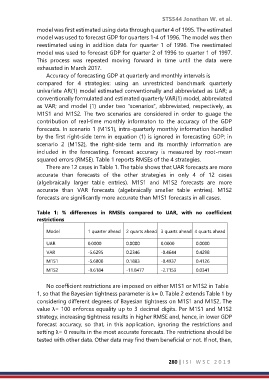
squared errors (RMSE). Table 1 reports RMSEs of the 4 strategies.
There are 12 cases in Table 1. The table shows that UAR forecasts are more
accurate than forecasts of the other strategies in only 4 of 12 cases
(algebraically larger table entries). M1S1 and M1S2 forecasts are more
accurate than VAR forecasts (algebraically smaller table entries). M1S2
forecasts are significantly more accurate than M1S1 forecasts in all cases.

Table 1: % differences in RMSEs compared to UAR, with no coefficient
restrictions

Model 1 quarter ahead 2 quarts ahead 3 quarts ahead 4 quarts ahead

UAR 0.0000 0.0000 0.0000 0.0000
VAR -5.6295 0.2346 -0.4644 0.4298
M1S1 -5.6800 0.1883 -0.4937 0.4126
M1S2 -9.6184 -11.8477 -2.7153 0.0341

No coefficient restrictions are imposed on either M1S1 or M1S2 in Table
1, so that the Bayesian tightness parameter is λ= 0. Table 2 extends Table 1 by
considering different degrees of Bayesian tightness on M1S1 and M1S2. The
value λ= 100 enforces equality up to 3 decimal digits. Per M1S1 and M1S2
strategy, increasing tightness results in higher RMSE and, hence, in lower GDP
forecast accuracy, so that, in this application, ignoring the restrictions and
setting λ= 0 results in the most accurate forecasts. The restrictions should be
tested with other data. Other data may find them beneficial or not. If not, then,

280 | I S I W S C 2 0 1 9