Page 443 - Special Topic Session (STS) - Volume 3

STS555 Patrice Bertail et al.
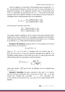
In the i.i.d. setting it is known that, if f is bounded by some constant Mf < +∞,
the corresponding functional is robust and may be simply estimated by its
empirical counterpart. In the Markovian situation, even in the bounded case,
(1)
T (b, LA) is generally not bounded and γ (T, LA) = ∞. This point has also been
∗
stressed in [4], with a different definition of the influence function however. A
robustified version of this parameter then can be defined as

and the plug-in estimator becomes

This simply consists in getting rid of the blocks (or the pseudo-blocks) whose
lengths are too large compared to M. This applies in particular to the estimation
of the stationary measure µ when f is an indicator function ∑ 1 { ≤ } leading
=1
˜
to an estimator FLA,M,n of the cdf of the stationary measures.
Example 2: M-estimators. Suppose that E ⊂ R for simplicity. Let θ be the
unique solution of the equation:

where g : R → R is of class C . Equipped with the notation g(b, θ) :=
2
2
∑ () (, ) for all b ∈ T, the score equation is equivalent to ELA [g(B, θ)] = 0. A
=1
calculation entirely similar to that carried out in the i.i.d. setting (provided that
differentiating inside the expectation is authorized) gives

()
where ∂g(b, θ)/∂θ = ∑ =1 (, )/. By definition of θ, we naturally have

Example 2: Quantiles. We place ourselves in the case E ⊂ R. Assume
that the stationary distribution has a continuous cdf Fµ(x) = µ(] − ∞, x]) and
density fµ(x). Consider the α−quantile This parameter can
also be viewed as a functional of LA, Tα(LA) say, it is the unique solution of the
equation

432 | I S I W S C 2 0 1 9