Page 444 - Special Topic Session (STS) - Volume 3

STS555 Patrice Bertail et al.

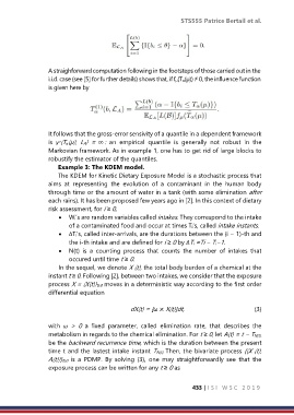
A straighforward computation following in the footsteps of those carried out in the
i.i.d. case (see [5] for further details) shows that, if fµ(Tα(µ)) ≠ 0, the influence function
is given here by

It follows that the gross-error sensivity of a quantile in a dependent framework
is γ (Tα(µ), LA) = ∞ : an empirical quantile is generally not robust in the
∗
Markovian framework. As in example 1, one has to get rid of large blocks to
robustify the estimator of the quantiles.
Example 3: The KDEM model.
The KDEM for Kinetic Dietary Exposure Model is a stochastic process that
aims at representing the evolution of a contaminant in the human body
through time or the amount of water in a tank (with some elimination after
each rains). It has been proposed few years ago in [2]. In this context of dietary
risk assessment, for i ≥ 0,
• Wi’s are random variables called intakes. They correspond to the intake
of a contaminated food and occur at times Ti’s, called intake instants.
• ΔTi’s, called inter-arrivals, are the durations between the (i − 1)-th and
the i-th intake and are defined for i ≥ 0 by ΔTi =Ti − Ti−1.
• N(t) is a counting process that counts the number of intakes that
occured until time t ≥ 0.
In the sequel, we denote X (t), the total body burden of a chemical at the
instant t ≥ 0. Following [2], between two intakes, we consider that the exposure
process X = (X(t))t≥0 moves in a deterministic way according to the first order
differential equation

dX(t) = [ω × X(t)]dt, (3)

with ω > 0 a fixed parameter, called elimination rate, that describes the

metabolism in regards to the chemical elimination. For t ≥ 0, let A(t) = t − TN(t),
be the backward recurrence time, which is the duration between the present
time t and the lastest intake instant TN(t). Then, the bivariate process {(X (t),
A(t))}t≥0 is a PDMP. By solving (3), one may straightforwardly see that the
exposure process can be written for any t ≥ 0 as

433 | I S I W S C 2 0 1 9