Page 156 - Special Topic Session (STS) - Volume 4

STS577 Mahdi Roozbeh
McKean, 1998, Ch.3):

T
a (R(y))Ha(R(y)), (2.4)

) , (()) = ((( )), … , ((( ))) , and ( ) is
where for = ( 1,…, 1 i
the rank of , = 1, . . . , , (1) ≤ (2) ≤ . . . ≤ () is a set of scores
generated as () = (/( + 1)) for some square-integrable and non-
decreasing score function () defined on the unit interval, satisfying

2
∫ ()d = 0 and ∫ ()d = 1,
− 1
and = ( ) is the projection matrix onto the space Ω , the

column space spanned by the columns of and = (X T , . . ., T T
X ) .
When the conditional distribution of i given is normal with < , the
classical test for Ho : β = 0 is the F-test. The F-statistic is a monotone function
of the likelihood ratio statistic and is distributed as a noncentral F distribution
under the alternative (Anderson, 2003). It is interesting to know the power
implication on the F-test when / → ∈ (0, 1) when both and diverge
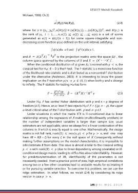
to infinity. The F-statistic for testing Ho has form

̂
̂

= , = ( ) −1 (2.5)

(−)
Under Ho, F has central Fisher distribution with and − degrees of
freedom (d.f.). Hence, an α- level F-test rejects Ho if F > f (p, n − p), the upper
α
α-level critical value of the F-distribution with p and n- p d.f.
Under situations in which the matrix X X is ill-conditioned due to linear
T
relationship among the regressors of X matrix (multicollinearity problem) or
the number of independent variables is larger than sample size, usual
estimators are not applicable, since we always find a linear combination of the
columns in X which is exactly equal to one other. Mathematically, the design
matrix is not full rank, () ≤ (, ) < for > , and one may
have Xβ = X(β + ζ) for every ζ in the null space of X. Consequently, without
making further assumptions on the model characteristics, it is impossible to
infer/estimate β from data. This issue is almost similar to the classical setting
< with () < (due to linear dependency among covariates) or ill-
conditioned design matrix, leading to difficulties about identifiability. However,
for prediction/estimation of Xβ, identifiability of the parameters is not
necessarily needed. From a practical point of view, high empirical correlations
among two or a few other covariates lead to unstable results for estimating β
or for pursuing variable selection. To overcome this problem, we can use the
ridge estimation. In what follows, we revisit (2.4) by considering its ridge
version in case > .

145 | I S I W S C 2 0 1 9