Page 397 - Special Topic Session (STS) - Volume 4

STS2320 Ali S. H.
experimental rule, a variable has a sever skewness if its absolute SC is greater
than 2 and severe kurtosis if its absolute value of KC is greater than 0.5.
What to do with variables that have severe skewness and/or kurtosis? One
way out here is to use the Box-Cox power transformation to make the variable
that have severe skewness and/or kurtosis closer to the Normal distribution.
To be specific, one can replace the i-th value, xi, by () = ∑ −1)/. The

parameter is chosen such that the distribution of the variable Y() is close to
normal. One way to achieve this is draw the Normal Probability Plot of Y()
and choose the value of that makes the graph as linear as possible.
Techniques such as the use of sliders (see, e.g., the software package Data
Desk) can be used to achieve this goal. Alternatively, the function
“BoxCoxLambda” in the R package “DescTools” automatically detects the
optimal parameter A. Note that if the optimal value of l turns out to be zero,
this indicates that the optimal transformation of the log transformation, that
is, y(0) = log(x).
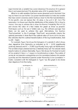
For example, Figure 1(a) shows the histogram of a variable X, which shows
clear departure from Normality as indicated by SC = 5.079 (significantly
positively skewed) and KC = 25.495 (significantly heavy right tail distribution).
The variable is highly skewed and has a relatively heavy tail. The variable needs
transformation to achieve Normality. Figure 1(b) shows the Normal Q-Q plot
of the variable X. Here = 1 means no transformation is taken. The scatter of
points do not resemble a straight line and the correlation between the sample
quantiles and the theoretical quantile (under Normality) is low (correlation =
0.544). Consistent with the histogram in Figure 1(a), this graph in (b) shows
clear departure from Normality.

Figure 1. Box-Cox Transformation of the variable X

386 | I S I W S C 2 0 1 9