Page 399 - Special Topic Session (STS) - Volume 4

STS2320 Ali S. H.
Another approach for the identification of univariate outliers is as follows:
The a% trimmed mean and trimmed standard deviation are computed based
on the central 100(1 – α)% of the values. Commonly used choices of a are 5%
and 10%. Then all observations more than 3 trimmed standard deviations away
from the trimmed mean are declared outliers. Outliers are then treated by
replacing them by

Trimmed mean – 3:1 x Trimmed standard deviation,

if they are in the lower tail, or by

Trimmed mean + 3:1 x Trimmed standard deviation,

if they are in the upper tail. This rule, which is simple and also strikes a balance
between efficiency and robustness, is adopted by other well-established
indices, such as the Ibrahim Index of African Governance (IIAG); see the MIF
foundation Web site at: mo.ibrahim.foundation.

3. The Multivariate Approach
Although the methods for the identification of univariate outliers are
simple and easy to compute, they may fail to identify outliers in higher-
dimensional spaces. For example, Figure 3 shows that scatter plot of two
variables Y and X. Here we can see clearly that there are two outliers in the
two-dimensional space. Neither one of the univariate methods for identifying
the outliers will identify these two observations because each one of then falls
near the mean of X and the mean of Y. An early method for the identification
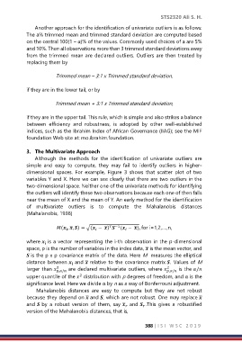
of multivariate outliers is to compute the Mahalanobis distances
(Mahalanobis, 1936)

−1
( , ̅, ) = √( − ̅) ( − ̅), for i=1,2,….,n,

where is a vector representing the i-th observation in the p-dimensional

space, p is the number of variables in the index data, ̅ is the mean vector, and
is the p x p covariance matrix of the data. Here M measures the elliptical
distance between and ̅ relative to the covariance matrix . Values of M

2
larger than ,/ are declared multivariate outliers, where 2 is the /
,/
upper quantile of the distribution with p degrees of freedom, and α is the
2
significance level. Here we divide α by n as a way of Bonferrouni adjustment.
Mahalanobis distances are easy to compute but they are not robust
because they depend on ̅ and , which are not robust. One may replace ̅
and by a robust version of them, say ̅ and .This gives a robustified

version of the Mahalanobis distances, that is,

388 | I S I W S C 2 0 1 9