Page 400 - Special Topic Session (STS) - Volume 4

STS2320 Ali S. H.

( , ̅ , ) = √( − ̅ ) ( − ̅), for i=1,2,….,n,
−1

Several methods exist for obtaining x r and S r. Two of the most common
ways are the Minimum Covariance Determinant (MCD) proposed, e.g., in
Rousseuw and Van Driessen (1999), and the Blocked Adaptive,
Computationally-Efficient outlier Numerator (BACON), proposed by Billor et
al. (2000). These two methods are implemented in R using the functions
“CovMcd” in the package “rrcov” and BACON in the Package “robustX”.
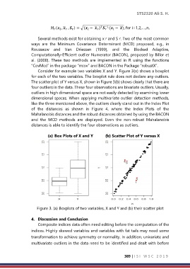
Consider for example two variables X and Y. Figure 3(a) shows a boxplot
for each of the two variables. The boxplot rule does not declare any outliers.
The scatter plot of Y versus X, shown in Figure 3(b) shows clearly that there are
four outliers in the data. These four observations are bivariate outliers. Usually,
outliers in high dimensional space are not easily detected by examining lower
dimensional spaces. When applying multivariate outlier detection methods,
like the three mentioned above, the outliers clearly stand out in the Index Plot
of the distances as shown in Figure 4, where the Index Plots of the
Mahalanobis distances and the robust distances obtained by using the BACON
and the MCD methods are displayed. Even the non-robust Mahalanobis
distances is able to identify the four observations as outliers.

(a) Box Plots of X and Y (b) Scatter Plot of Y versus X

Figure 3. (a) Boxplots of two variables, X and Y and (b) their scatter plot

4. Discussion and Conclusion
Composite indices data often need editing before the computation of the
indices. Highly skewed variables and variables with fat tails may need some
transformation to achieve symmetry or normality. In addition, univariate and
multivariate outliers in the data need to be identified and dealt with before

389 | I S I W S C 2 0 1 9