Page 330 - Contributed Paper Session (CPS) - Volume 2

CPS1876 Sarbojit R. et al.
literature that improve the performance of the NN classifier in HDLSS
settings. Chan and Hall (2009) developed some scale adjustments to the usual
1NN classifier, and this method performs well under the weaker condition that
2
12 > 0. A non-linear transformation of covariate space followed by the 1NN
classification was proposed by Dutta and Ghosh (2016). Recently, Pal et al.
(2016) used a new dissimilarity index instead of the usual Euclidean distance
for 1NN classification. However, all these methods require either of the
2
2
2
conditions 12 > 0 or ≠ to yield good results for high-dimensional data.
1
2
So, they can deal with distributions that differ either in their locations or scales.
Consider a two class classification problem (say, Example 1) with the
competing distributions as ≡ ( , ∑ (1) ) and ≡ ( , ∑ (2) ). Here,

1

2

denotes the − dimensional Gaussian distribution, is the
−dimensional vector of zeros, and ∑ (1) and ∑ (2) are described below:

0.5
(1) [ ] [ ]×(−[ ]) (2) −[ ] (−[ ])×[ ]
2
2
2
2
2
2
∑ = [ ] and ∑ = [ ] ,
0.5
(−[ ])×[ ] −[ ] [ ]×(−[ ]) [ ]
2 2 2 2 2 2

with being the × identity matrix and × being the × matrix of

5
zeros. As Example 2, we consider ≡ ( , ) and ≡ ∏ with

1
=1
2

2
3
2 = (0,1) for each 1 ≤ ≤ . Throughout this article, we follow the
5

convention that if we write = ( , … , ) ~ , then ~ for all 1 ≤ ≤

1

2
2
2
. It is easy to check that 12 = 0 and = = 0.75 for Example 1. For
2
1
5
Example 2, the parameters are (1) = (2) = and ∑ (1) = ∑ (2) = ,

3
2
2
2
hence we obtain 12 = 0 and = = 5 . Despite having different
2
1
3
2
2
2
populations, both these examples end up with 12 = 0 and = . The
2
1
existing NN classifiers fail to yield promising results in high-dimensional
spaces. Similar arguments hold for any in the NN classifier as → ∞ (with
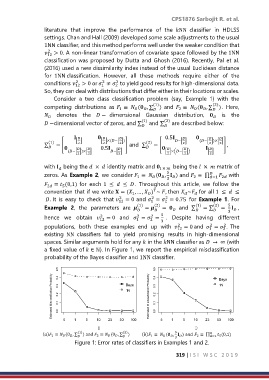
a fixed value of ∈ ℕ). In Figure 1, we report the empirical misclassification
probability of the Bayes classifier and 1NN classifier.

(1) (2) 5
() 1 ≡ (0 , ∑ ) and 2 ≡ (0 , ∑ ) () 1 ≡ ( , ) and 2 ≡ ∏ 5 (0,1)
3 =1
Figure 1: Error rates of classifiers in Examples 1 and 2.
319 | I S I W S C 2 0 1 9