Page 333 - Contributed Paper Session (CPS) - Volume 2

CPS1876 Sarbojit R. et al.
1
2, yields good performance. In fact, under certain assumptions, we proved
that ∆ 1 2, converges to zero as → ∞.

3. Identifying Joint Structures
In Section 2, we observed that the NN classifier based on 2, (namely,

2, ) can discriminate populations that have difference in their one-
dimensional marginal distributions. But, if the one-dimensional marginals are
same, gMADD will fail to differentiate between populations. Such scenarios
1
impose further challenges on the proposed classifier 2, . Consider two class
(1) (2)
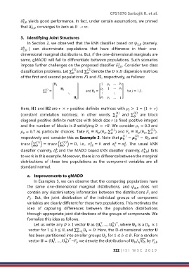
classification problems. Let ∑ and ∑ denote the × dispersion matrices
of the first and second populations F1 and F2, respectively, as follows:

1 …

() 1 …
∑ = and = for = 1,2.
⋮
⋱ ⋱
[ ] [ … 1 ]

Here, 1 and 2 are × positive definite matrices with > 1 = (1 + )

(1) (2)
(constant correlation matrices). In other words, ∑ and ∑ are block
diagonal positive definite matrices with block size (a fixed positive integer)
and the number of blocks is satisfying = . We consider = 0.3 and
1
(1) (2)
= 0.7 as particular choices. Take ≡ (0 , ∑ ) and ≡ (0 , ∑ ),
1

2
2

respectively and consider this as Example 3. Note that (1) = (2) = and

2
2
2
(∑ (1) ) = (∑ (2) ) = , i.e., 12 = 0 and = . The usual NN
1
2

classifier (namely, and the MADD based NN classifier (namely, 1, ) fails

to work in this example. Moreover, there is no difference between the marginal
distributions of these two populations as the component variables are all
standard normal.

a. Improvements to gMADD
In Examples 3, we can observe that the competing populations have
the same one-dimensional marginal distributions, and 2, does not
contain any discriminatory information between the distributions and
1
. But, the joint distribution of the individual groups of component
2
variables are clearly different for these two populations. This motivates the
idea of capturing differences between the population distributions
through appropriate joint distributions of the groups of components. We
formalize this idea as follows.
Let us write any × 1 vector as ( , … , ) , where is a D × 1
⊤
⊤ ⊤
1

vector for 1 ≤ ≤ , and ∑ = . Here, the D-dimensional vector
=1
has been partitioned into smaller groups for 1 ≤ ≤ . For a random

vector = ( , … , ) ~ , we denote the distribution of /√ by
⊤
⊤ ⊤
,

1

322 | I S I W S C 2 0 1 9