Page 336 - Contributed Paper Session (CPS) - Volume 2

CPS1876 Sarbojit R. et al.
have also been studied, and the respective misclassifiction rates are
reported as well
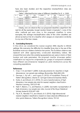
Table 1: Misclassification rates of different classifiers for = 1000
Ex. Bayes NN- NN- GLMNET RF NN- SVM-LIN SVM-
gMADD ggMADD RAND RBF
1 0.00(0.00) 0.00(0.00) - 0.47(0.02) 0.01(0.01) 0.40(0.02) 0.37(0.02) 0.36(0.02)
2 0.00(0.00) 0.04(0.01) - 0.47(0.02) 0.35(0.02) 0.50(0.02) 0.37(0.02) 0.38(0.02)
3 0.00(0.00) 0.44(0.02) 0.02(0.01) 0.48(0.02) 0.49(0.02) 0.50(0.02) 0.51(0.00) 0.47(0.00)
4 0.00(0.00) 0.48(0.02) 0.20(0.03) 0.47(0.01) 0.49(0.02) 0.49(0.02) 0.50(0.02) 0.49(0.02)

Clearly, one can observe that our proposed classifiers outperform the
rest for all the examples. Except random forest in Example 1, none of the
other methods get even close to the proposed classifiers. In some
examples, the average misclassification rates of the other classifiers are
almost as bad as that of a classifier which assigns an observation randomly
to any one of the two classes.

5. Concluding Remarks
In this article, we considered the nearest neighbor (NN) classifier in HDLSS
settings. We overcame the difficulty this classifier faces due to the use of the
Euclidean norm as a distance between two points. The Euclidean distance was
replaced with other appropriately constructed dissimilarity indices. We
showed that even when the underlying populations are same in terms of their
location and scale parameters, the proposed classifier showcases perfect
classification as long as the components (or, groups of component variables)
have different one-dimensional marginal (or, joint) distributions across the
competing populations.

References
1. Chan, Y.-B. and Hall, P. (2009). Scale adjustments for classifiers in high-
dimensional, low sample size settings. Biometrika, 96(2):469–478.
2. Devroye, L., Gy¨orfi, L., and Lugosi, G. (2013). A Probabilistic Theory of
Pattern Recognition, volume 31. Springer Science & Business Media.
3. Dutta, S. and Ghosh, A. K. (2016). On some transformations of high
dimension, low sample size data for nearest neighbor classification.
Machine Learning, 102(1):57–83.
4. Hall, P., Marron, J. S., and Neeman, A. (2005). Geometric representation of
high dimension, low sample size data. Journal of the Royal Statistical
Society Series B, 67(3):427–444.
5. Pal, A. K., Mondal, P. K., and Ghosh, A. K. (2016). High dimensional
nearest neighbor classification based on mean absolute differences of
inter-point distances. Pattern Recognition Letters, 74:1–8.

325 | I S I W S C 2 0 1 9