Page 360 - Contributed Paper Session (CPS) - Volume 2

CPS1887 Sahidan A. et al.
3. Result
LST data was used to analyze the seasonal pattern and trend of average
increase. The data was applied from 2000 to 2018. Before downloading the
data, we divided the area into region which consists of eight super-regions.
2
Each super-region includes nine sub-region with the area of 7×7 km . Every
2
region had an area 52×52 km with 1×1 km grids. Therefore, there are 72
2
sub-regions. Firstly, we created the first model and fit spline which consists
of eight knots in order to see the seasonal patterns for each super-region.
The temperature that given from MODIS was in kelvin but, we used to
convert from Kelvin to Celsius by minus 273.15. This is because Celsius is a
common scale and unit of measurement for temperature. Then, we plot the
day temperature data of each sub-region in order to get the seasonal
pattern of each super region as below:

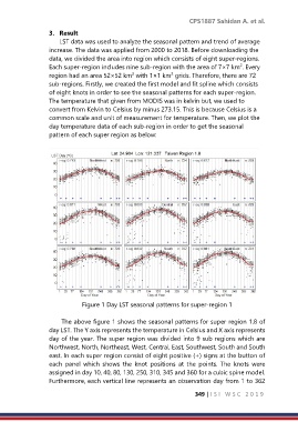
Figure 1 Day LST seasonal patterns for super-region 1

The above figure 1 shows the seasonal patterns for super region 1.8 of
day LST. The Y axis represents the temperature in Celsius and X axis represents
day of the year. The super region was divided into 9 sub regions which are
Northwest, North, Northeast, West, Central, East, Southwest, South and South
east. In each super region consist of eight positive (+) signs at the button of
each panel which shows the knot positions at the points. The knots were
assigned in day 10, 40, 80, 130, 250, 310, 345 and 360 for a cubic spine model.
Furthermore, each vertical line represents an observation day from 1 to 362

349 | I S I W S C 2 0 1 9