Page 386 - Contributed Paper Session (CPS) - Volume 2

CPS1891 Tzee-Ming Huang
(iii) Compute the BIC (Bayesian information criterion) for the model in
(2) by taking { , … , } to be and = 3.
1

• Choose the with the smallest BIC value as the final set of selected

knots.
Note that in Algorithm 1, (7) may not hold with = 1/2 for all . However,

if is large enough, then (7) holds with = 1/2 for large enough j. in such

case, there is a chance that proper knots are selected based on the screening
test. In the simulation experiment in Section 3, is taken to be 5.

3. Result
A simulation experiment has been carried out to examine the performance
of the proposed algorithm and the results are given in this section.
For the simulation experiment, the data generating process is described

below. 100 data sets are generated from model (1) with = 2000, = /( −

1) for = 0,1, … , − 1, s are IID N(0, ) , and ∈ { , , , }, where
2

3
1
2
4
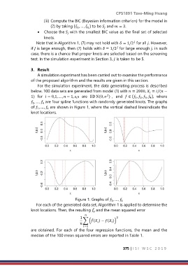
, … , are four spline functions with randomly generated knots. The graphs
1
4
of , … , are shown in Figure 1, where the vertical dashed linesindicate the
4
1
knot locations.

Figure 1: Graphs of , … ,
1
4
For each of the generated data set, Algorithm 1 is applied to determine the
knot locations. Then, the resulting and the mean squared error
̂
s

1 ∑ (( ) − ( ))
2
̂

=1
are obtained. For each of the four regression functions, the mean and the
median of the 100 mean squared errors are reported in Table 1.
375 | I S I W S C 2 0 1 9