Page 55 - Contributed Paper Session (CPS) - Volume 2

CPS1419 Jinheum K. et al.
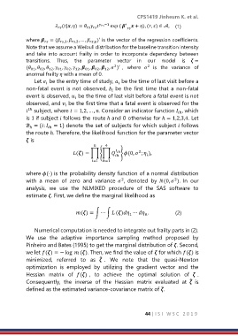
(|, ) = −1 exp ( ′ + ), (, ) ∈ , (1)

′
where = ( ,1 , ,2 , … , , ) is the vector of the regression coefficients.
Note that we assume a Weibull distribution for the baseline transition intensity
and take into account frailty in order to incorporate dependency between
transitions. Thus, the parameter vector in our model is =
( , , , , , , , , , ) , where is the variance of
2 ′
2
01
12
01
02
02
12
01
02
12
anormal frailty with a mean of 0.
Let be the entry time of study, be the time of last visit before a

non-fatal event is not observed, be the first time that a non-fatal

event is observed, be the time of last visit before a fatal event is not

observed, and be the first time that a fatal event is observed for the

subject, where = 1,2, … , . Consider an indicator function , which
ℎ
ℎ
is 1 if subject follows the route ℎ and 0 otherwise for ℎ = 1,2,3,4. Let
ℬ = {: = 1} denote the set of subjects for which subject follows
ℎ
ℎ
the route ℎ. Therefore, the likelihood function for the parameter vector
is
4
() = ∏ {∏ } (0, ; ),
2
ℎ
ℎ
=1 ℎ=1

where (⋅) is the probability density function of a normal distribution
with a mean of zero and variance , denoted by (0, ). In our
2
2
analysis, we use the NLMIXED procedure of the SAS software to
estimate . First, we define the marginal likelihood as

() = ∫ ⋯ ∫ () ⋯ . (2)

1

Numerical computation is needed to integrate out frailty parts in (2).
We use the adaptive importance sampling method proposed by
Pinheiro and Bates (1995) to get the marginal distribution of . Second,
we let () = − log (). Then, we find the value of for which () is
minimized, referred to as . We note that the quasi-Newton
̂
optimization is employed by utilizing the gradient vector and the
Hessian matrix of () , to achieve the optimal solution of .
Consequently, the inverse of the Hessian matrix evaluated at is
̂
defined as the estimated variance-covariance matrix of .
̂

44 | I S I W S C 2 0 1 9