Page 263 - Contributed Paper Session (CPS) - Volume 4

CPS2220 David Degras et al.
= +

(3)
+ , 1 ≤ ≤
= ∑ (−ℓ)

ℓ
ℓ=1
Following [10], we refer to model (3) as the switching observations model.
Here, both the observation matrix and observed state vector depend on the
regime . There are in fact different state vectors , 1 ≤ ≤ , evolving

independently according to a VAR() model determined by the and . At
ℓ
time , only one of these state vectors is observed through . Dependencies

between observations, state vectors, and regimes under this model are
depicted in Figure 1 (right panel). Model (3) can be viewed as a mixture-of-
experts neural network wherein the SSMs specified by = + and

= ∑ (−ℓ) + (1 ≤ ≤ ) are experts and ( ) is a gating network

ℓ

ℓ=1
[4].

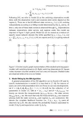
Figure 1: Directed acyclic graph representation of the studied switching space-
models. Left: switching dynamics (2). Right: switching observations (3). Square
nodes represent discrete variables and oval ones are Gaussian. Shaded nodes
are observed while white one are hidden.

3. Model fitting by the EM algorithm
A general presentation of the EM algorithm can be found in [9] and its
specific implementation in model (1) is described in [7, 10]. For reasons of
space, we omit a full presentation here and focus on our new developments.
Let = {( , , , , , ∑ ) ∶ 1 ≤ ≤ ; ; } be the collection of all

parameters in model (1), with = ( , … , )ˊ and = ( ) For

1
1≤,≤.
brevity we denote the measurements ( ) 1: , the state vectors
1≤≤ by
() 1≤≤ by 1: , etc. We recall that only the measurements 1: are observed
whereas both the state vectors 1: and regimes 1: are unobserved. We
denote the complete likelihood function (i.e., if 1: , 1: , 1: were all
observed) by (). We also denote the probability measure associated to

model (1) by and expectation under by .

252 | I S I W S C 2 0 1 9