Page 84 - Contributed Paper Session (CPS) - Volume 1

CPS1110 Selamawit M. et al.
observations provide the bi-variate display in Fig. 1b, where the colors of the
points corresponds to the soil classes. The points for some soil classes appear
in more than one cluster, which indicates a bimodal likelihood model ( | ).

In Moja et al. (2018) a Gaussian likelihood model is assumed which does not
capture bimodality, see Fig.1b.
Consider the likelihood model (|) as a pdf of ∈ given ∈ Ω ,

2
and denote the related observations = ( , · · · , ). Then (|)

1
2

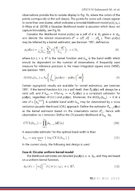
may be inferred by a kernel-estimator, see Izenman 1991, defined as:

where ( ); ∈ is the kernel function and ℎ is the band width which
2

should be dependent on the number of observations. A frequently used
measure for inference precision is the mean integrated square error (MISE),
see Izenman 1991,

Certain asymptotic results are available for kernel estimators, see Izenman
1991. If the kernel function ( ) is a pdf itself, then (|) will always be a
̂

̂
valid pdf, and if ℎ → 0 for → ∞, (|) is a consistent estimator for

(|), regardless of ( ) and (|). Moreover, the (ℎ ) → 0 at a

−1/3
rate of ( ). A suitable band width ℎ may be determined by a cross

̂
validation psuedo-likelihood (CVL) approach. Define the estimator (|)
(−)
as the kernel estimator based on the observation vector , hence with

−
observation no removed. Define the CV psuedo-likelihood of ℎ by,

A reasonable estimator for the optimal band width is then

In the current study, the following test design is used:

Case A: Circular uniform kernel model
The likelihood estimates are denoted ̂(|): ∈ Ω , and they are based

on a uniform kernel function,

73 | I S I W S C 2 0 1 9