Page 23 - Contributed Paper Session (CPS) - Volume 2

CPS1408 Caston S. et al.
electricity prices are developed by Gaillard et al. [4]. The work done by Gaillard
et al. [4] is extended by Fasiolo et al. [3] who developed fast calibrated additive
quantile regression models. An online load forecasting system for very-short-
term load forecasts is proposed by Laouafi et al. [7]. The proposed system is
based on a forecast combination methodology which gives accurate forecasts
in both normal and anomalous conditions. Zhang et al. [11] developed a
hybrid model to short-term load forecasting based on singular spectrum
analysis and support vector machine which is optimized by the heuristic
method they refer to as the Cuckoo search algorithm. The new proposed
model outperformed the other heuristic models used in the study.
Joint modelling of hourly electricity demand using additive quantile
regression with pairwise inter- actions including an application of quantile
regression averaging (QRA) is not discussed in detail in the literature. The
current study intends to bridge this gap. The study focuses on an application
of additive quantile regression (AQR) models. A comparative analysis is then
done with the generalized additive models (GAMs) which are used as
benchmark models. In this study we discuss an application of pairwise
hierarchical interactions discussed in Bien et al. [2] and Laurinec [8] who
showed that the inclusion of interactions improves forecast accuracy. A
discussion of the models is presented in Section 2, with Section 3 discussing
the results of the study. The conclusion is given in Section 4.

2. Models

2.1 Additive quantile regression model
An additive quantile regression (AQR) model is a hybrid model which is a
combination of GAM and QR models. AQR models were first applied to short-
term load forecasting by Gaillard et al. [4] and extended by Fasiolo et al. [3].
Let t denote hourly electricity demand where t = 1,...,n, n is the number of

observations and let the number of days be denoted by nd. Then n = 24nd
where 24 is the number of hours in a day and the corresponding p
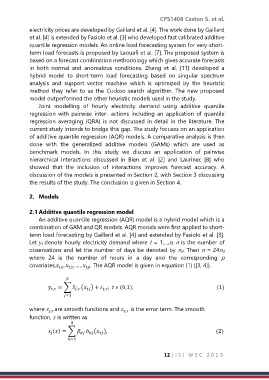
covariates, , , … , . The AQR model is given in equation (1) ([3, 4]).

2
1

y , = ∑ ( ) + ; (0,1), (1)
,
,

=1

where are smooth functions and , is the error term. The smooth
,
function, is written as

() = ∑ ( ), (2)

=1
12 | I S I W S C 2 0 1 9