Page 25 - Contributed Paper Session (CPS) - Volume 2

CPS1408 Caston S. et al.
2.4 Forecast combination
QRA is based on forecasting the response variable against the combined
forecasts which are treated as independent variables. QRA was first introduced
by Nowotarski and Weron ([10]). Let , be hourly electricity demand as
discussed in Section 2.1 and let there be M methods used to predict the next
observations of which shall be denoted by +1 , +2 , … , + . Using m =
,
1,...,M methods, the combined forecasts will be given by

̂ , = + ∑ ̂ + , (7)
0
,

=1

where ̂ , represents forecasts from method , ̂ , is the combined
forecasts and , is the error term. We seek to minimise

min ∑ (̂ − − ∑ ̂ ). (8)

0

=1 =1

3. Empirical Result
3.1 Forecasting results
The data used is hourly electricity demand from 1 January 2010 to 31
December 2012 giving us n = 26281 observations. The data is split into
training data, 1 January 2010 to 2 April 2012, i.e. n1 = 19708 and testing data,
from 2 April 2012 to 31 December 2012, i.e. n2 = 6573, which is 25% of the
total number of observations. The models considered are M1 (GAM), M2 (GAMI)

which are GAM models without and with interactions respectively, and M3
(AQR), M4 (AQRI) which are additive quantile regression models without and
with interactions, respectively. The four models M1 to M4 are then combined
based on the pinball losses, resulting in M5 and also combined using QRA,
resulting in M6.
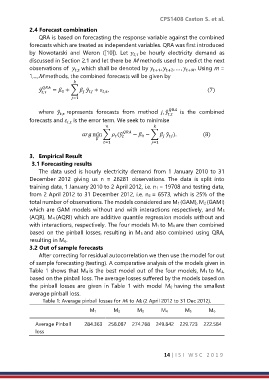
3.2 Out of sample forecasts
After correcting for residual autocorrelation we then use the model for out
of sample forecasting (testing). A comparative analysis of the models given in
Table 1 shows that M4 is the best model out of the four models, M1 to M4,
based on the pinball loss. The average losses suffered by the models based on
the pinball losses are given in Table 1 with model M6 having the smallest
average pinball loss.
Table 1: Average pinball losses for M1 to M6 (2 April 2012 to 31 Dec 2012).
M1 M2 M3 M4 M5 M6

Average Pinball 284.363 258.087 274.768 249.842 229.723 222.584
loss

14 | I S I W S C 2 0 1 9