Page 64 - Contributed Paper Session (CPS) - Volume 2

CPS1428 Enobong F. U.
( )

( + 1) ( ) − 1
= ( )⁄ ( )
( )

( + 1) ( ) − 1
( )
=

( + 1)
α=

x a

lnR(x b )

(e Q +1) lnR(x a ) ‐1
ln
lnR(x b ) lnR(x m ) lnR(x b ) lnR(x b )

x b
x b
Q
Q
Q
‐ {ln [(e +1) lnR(x a ) ‐1] ln ( x m )‐ln ( ) ln [(e +1) lnR(x a ) ‐1] +ln ( ) ln [(e +1) lnR(x a ) ‐1]} e { [(e Q +1) lnR(x a ) ‐1] }
⁄
x b x a x a

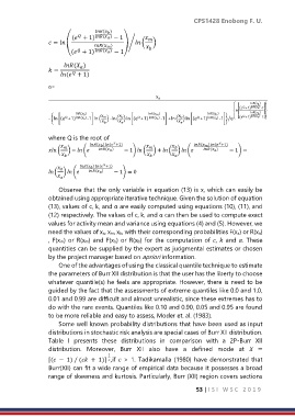
where Q is the root of

( ) ( +1) ( ) ( +1)
( ) − ( ( ) − 1) ( ) + ( ) ( ( ) − 1) −

( ) ( +1)
( ) ( ( ) − 1) = 0

Observe that the only variable in equation (13) is x, which can easily be
obtained using appropriate iterative technique. Given the solution of equation
(13), values of c, k, and α are easily computed using equations (10), (11), and
(12) respectively. The values of c, k, and α can then be used to compute exact
values for activity mean and variance using equations (4) and (5). However, we
need the values of xa, xm, xb, with their corresponding probabilities F(xa) or R(xa)
, F(xm) or R(xm) and F(xb) or R(xb) for the computation of , and . These
quantities can be supplied by the expert as judgmental estimates or chosen
by the project manager based on apriori information.
One of the advantages of using the classical quantile technique to estimate
the parameters of Burr XII distribution is that the user has the liberty to choose
whatever quantile(s) he feels are appropriate. However, there is need to be
guided by the fact that the assessments of extreme quantiles like 0.0 and 1.0,
0.01 and 0.99 are difficult and almost unrealistic, since these extremes has to
do with the rare events. Quantiles like 0.10 and 0.90, 0.05 and 0.95 are found
to be more reliable and easy to assess, Moder et. al. (1983).
Some well known probability distributions that have been used as input
distributions in stochastic risk analysis are special cases of Burr XII distribution.
Table I presents these distributions in comparison with a 2P-Burr XII

distribution. Moreover, Burr XII also have a defined mode at =
1
[( − 1) ⁄ ( + 1)] ,if > 1. Tadikamalla (1980) have demonstrated that
Burr(XII) can fit a wide range of empirical data because it possesses a broad
range of skewness and kurtosis. Particularly, Burr (XII) region covers sections

53 | I S I W S C 2 0 1 9