Page 276 - Contributed Paper Session (CPS) - Volume 6

CPS1929 Takayuki M.
Furthermore, we also assume that:

where Et−1[·] is the expectation at time t − 1 given the observations until time
t − 1. Then we have with ξt ∼ N(0,In. We refer to gi and mi as the
short and long run variance components respectively for asset i and denote
by Nv the number of days that mi is held fixed. The superscript i indicates that
i
this may be asset-specific and the subscript v differentiates it from a similar
scheme that will be introduced later for correlations. In particular, while gi,t
moves daily, mi,τ changes only once every Nv days. We assume that for each
i
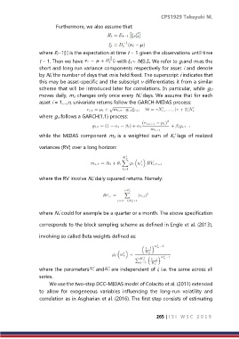
asset i = 1,...,n, univariate returns follow the GARCH-MIDAS process:

where gi,t follows a GARCH(1,1) process:

i
while the MIDAS component mi,τ is a weighted sum of Kv lags of realized
variances (RV) over a long horizon:

i
where the RV involve Nv daily squared returns. Namely:

i
where Nv could for example be a quarter or a month. The above specification
corresponds to the block sampling scheme as defined in Engle et al. (2013),

involving so called Beta weights defined as:

where the parameters and are independent of i, i.e. the same across all
series.
We use the two-step DCC-MIDAS model of Colacito et al. (2011) extended
to allow for exogeneous variables influencing the long-run volatility and
correlation as in Asgharian et al. (2016). The first step consists of estimating

265 | I S I W S C 2 0 1 9